Orthogonal vectors have zero inner product. See why perpendicular factor loadings can still produce correlated returns, and why scaling and the zero vector matter.
Orthogonal vectors
Orthogonal vectors have zero inner product. For real vectors in the usual Euclidean geometry, this means their dot product is zero:
a⊥b⟺aTb=i=1∑naibi=0.
When both vectors are nonzero, they meet at a right angle. In quantitative finance, this geometry helps separate factor directions, construct residuals and simplify risk calculations. But the phrase “orthogonal strategies” is incomplete until we know which vectors and which inner product are being used. Perpendicular loading vectors need not produce uncorrelated returns.
What disappears at a right angle
Take two dimensionless vectors in the same reference coordinates:
a=(1,1),b=(1,−1).
Their coordinate products cancel: aTb=1−1=0. Each has Euclidean norm2, so the angle formula gives
cosθ=∥a∥2∥b∥2aTb=0,θ=90∘.
The useful consequence is the disappearance of the cross term:
∥a+b∥22=∥a∥22+2aTb+∥b∥22=2+0+2=4.
Indeed, a+b=(2,0) has length 2. This is Pythagoras expressed through a dot product, and it works in any finite dimension.
Orthogonal does not mean unit length. Dividing each vector above by 2 makes them an orthonormal basis of the plane: perpendicular and unit length. More generally, mutually orthogonal nonzero vectors are linearly independent. Taking the inner product of ∑icivi=0 with vj isolates cj∥vj∥2=0, forcing every coefficient to vanish.
The nonzero condition matters. The zero vector is orthogonal to every vector because every coordinate product is zero. It has no direction, makes the angle formula undefined and cannot belong to a basis. Orthogonality does not license dividing by a zero norm.
Two perpendicular loading vectors, two correlated books
Suppose F1,F2 are synthetic, zero-mean factor returns over one common period, expressed as decimal returns. Two books have linear factor-return contributions
RA=F1+F2=aTF,RB=F1−F2=bTF.
Here F=(F1,F2)T. Loadings measure exposure per unit of the same reference capital; they are not constrained to sum to one. Assume the factor covariance matrix is
Σ=(0.040.010.010.09).
The books' covariance is determined by the factor distribution:
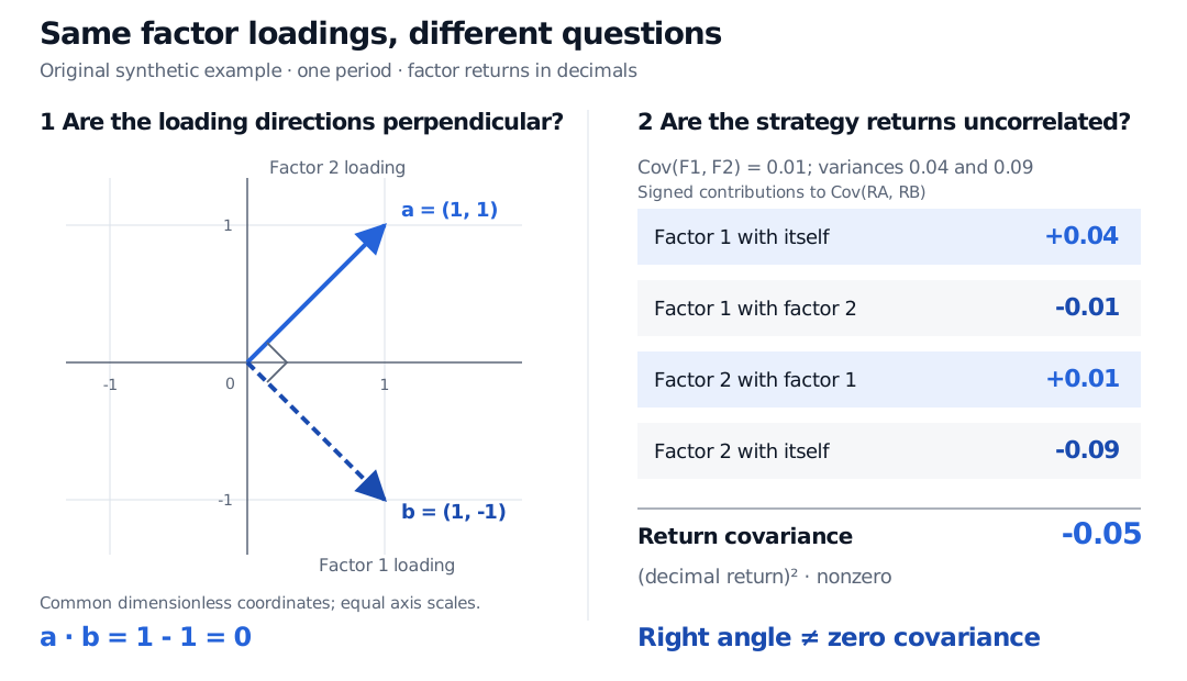
Cov(RA,RB)=aTΣb=0.04−0.01+0.01−0.09=−0.05.
The units are squared decimal returns for that period. Equivalently, expand Cov(F1+F2,F1−F2): the two mixed covariance terms cancel, leaving Var(F1)−Var(F2). The factor variances differ, so the answer is nonzero despite the right angle between the loadings.
Synthetic factor loadings a=(1,1) and b=(1,-1) meet at a right angle on equal-scale dimensionless axes. A separate ledger of loading-weighted covariance terms gives 0.04 minus 0.01 plus 0.01 minus 0.09, equalling negative 0.05 squared decimal returns.
Original synthetic, one-period factor model. The left panel tests Euclidean loading geometry; the right panel uses the specified factor covariance matrix to test return co-movement.
For completeness, the two book variances are aTΣa=0.15 and bTΣb=0.11. Their correlation is therefore −0.05/0.15×0.11≈−0.3892, rather than zero. These are model inputs and consequences, not estimated market relationships.
State the geometry before using the conclusion
An inner product specifies what “perpendicular” means. For a symmetric positive definite matrix M, the rule
⟨x,y⟩M=xTMy
defines a different geometry. Taking M=Σ in the example makes orthogonality of loading vectors mean zero covariance of the corresponding book returns. The displayed Σ is positive definite; if a covariance matrix is only positive semidefinite, this rule can give a nonzero loading zero length and is not an inner product on the full loading space.
The ordinary dot product gives that same zero-covariance test when the factors are uncorrelated and have a common positive variance: Σ=σ2I. Without that assumption, ordinary perpendicularity of loadings is insufficient.
Coordinate scaling also matters. Multiply the first coordinate of both example vectors by 2: the resulting vectors (2,1) and (2,−1) have ordinary dot product 4−1=3. Applying an unchanged Euclidean rule after unequal coordinate rescaling changes the geometry. If this is only a re-expression of the same geometric objects, the inner-product formula must change with the coordinates. Financial axes with different units or arbitrary scales need an explicit normalisation or metric before their angles have a useful interpretation.
A different construction applies when vectors contain observed returns across dates rather than factor loadings across factors. With equally weighted observations aligned and each series demeaned, their dot product is the numerator of sample covariance; its zero then means zero sample covariance. Demeaning and the observation weights are part of that statement. Raw returns do not inherit it automatically.
Even zero return covariance does not generally imply statistical independence, nor does an in-sample orthogonality constraint guarantee future co-movement will remain zero. Orthogonality is exact relative to a specified geometry and data set; its economic interpretation needs the corresponding model assumptions.
This same idea drives orthogonal projection: remove the component along a chosen direction or subspace, leaving a perpendicular residual. For the example pair, projection of a onto b is zero in Euclidean geometry, even though the books' return covariance is not.
Expectation, Variance and Covariance supplies the probabilistic definitions, diversification formula and distinction between uncorrelated and independent. The complete lesson is available with a free signed-in account; the public page is a preview.
Sources
Gilbert Strang, Introduction to Linear Algebra, 5th edition, Wellesley–Cambridge Press, 2016, §4.1, “Orthogonality of the Four Subspaces,” pp. 194–195: dot-product orthogonality and the Pythagorean identity.