Derivative pricing values contractual payments today. An exact stock-and-bank hedge explains no-arbitrage value, pricing probabilities and the limits of replication.
Derivative pricing
Derivative pricing assigns a present value to a financial contract's future payments and rights, using its terms, observable market inputs and valuation assumptions. A desk uses that value to quote a trade, mark an existing position and work out a hedge. The central question is what today’s traded assets imply about the contract’s payments—not simply whether the underlying asset is likely to rise.
The output needs a label. For a call option, the price is a premium paid for a right. For a new forward contract, “pricing” often means choosing the delivery price that makes the contract’s initial value zero. A delivery price and the present value of an existing forward are different quantities. A swap similarly involves a schedule of exchanged payments, rather than one option payoff.
A price forced by two possible payments
Consider an original synthetic market with just today and one future payment date. A non-dividend-paying share costs 100 USD today and will be worth either 120 or 80 USD then. Both states are possible. One unit of money in the risk-free bank account becomes 1.05 units over this entire period: a 5% return per period, with no annualization assumed.
The contract is a European call covering one share, with strike 100 USD. Its cash-equivalent payoff at the payment date is 20 USD in the up state and zero in the down state.
Assume frictionless trading: divisible holdings, no taxes or trading costs, freely available borrowing and lending at that same 1.05 gross rate, and the ability to buy or short the stock and derivative. There are no dividends, default, collateral restrictions or intervening payments. Positions can be held to settlement. These are assumptions of this two-state model.
Construct a replicating portfolio: hold Δ shares and an initial bank balance B0, where a negative balance means debt. Matching both terminal payments requires
120Δ+1.05B080Δ+1.05B0=20,=0.
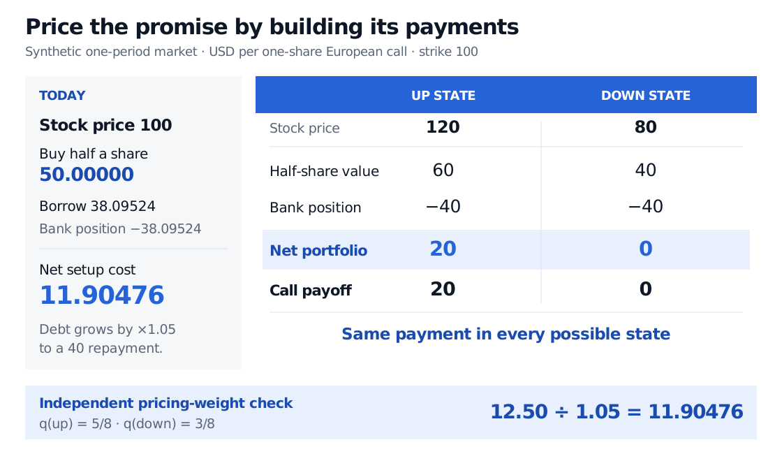
Subtracting the equations gives Δ=1/2. The down-state equation then requires B0=−40/1.05=−800/21. Buy half a share for 50 USD and borrow approximately 38.09524 USD. The net cost is
V0=100Δ+B0=50−21800=21250≈11.90476 USD.
Two-state derivative-pricing ledger: half a share costs 50 USD and borrowing supplies 38.09524 USD, for a net cost of 11.90476 USD. Terminal half-share values of 60 or 40 less debt of 40 give 20 or zero, matching the strike-100 call.
Original synthetic one-period ledger, in USD per one-share call. The bank balance grows at gross rate 1.05; the terminal portfolio matches the call in each possible state.
The law of one price makes this the call’s unique no-arbitrage value inside the model. The hedge duplicates each payment, so a different price creates a tradable discrepancy. If the call were quoted at 13 USD, shorting it and buying the replica would leave 13−250/21=23/21 USD today. Lending that excess produces 1.15 USD at settlement, while the call obligation and the replicating portfolio cancel in either state. The construction depends on the stated trading and funding permissions.
The probability comes from prices
No forecast probability appeared in the replication equations. The same answer can be expressed through a risk-neutral probabilityq, chosen so that the stock’s weighted terminal value equals its current price grown at the bank rate:
120q+80(1−q)=100(1.05),q=120−80105−80=85.
The up-state pricing weight is 62.5%; the down-state weight is 37.5%. Because 80<105<120, both weights are strictly between zero and one. Risk-neutral valuation now gives
V0=1.05q(20)+(1−q)(0)=1.0512.50=21250 USD.
The 12.50 USD numerator is an expected payoff under the pricing weights, not a prediction of the payment. The actual up-move probability can differ from 62.5% without changing this model price when the traded prices, two possible outcomes and funding terms stay fixed. Discounting an arbitrary physical expected payoff at the risk-free rate would generally break the replication identity.
For the fuller derivation and extension to a recombining tree, The Binomial Model is a complete public sample lesson, available without an account.
Where the unique answer stops
This market is complete: the two independent traded payoff vectors—stock and bank account—span every pair of payments in its two states. That is why the hedge determines one price. It does not establish that every real derivative can be replicated perfectly.
In an incomplete market, some risks cannot be eliminated with the available trades. No-arbitrage can then permit several values for an unspanned claim; selecting one can require additional assumptions about risk prices or calibration to other traded claims. Even a replicable model can have model risk when its states and dynamics describe the market poorly. Trading costs, discrete hedging, financing differences and counterparty terms also affect what an executable quote requires.
For an actual valuation, first specify the payments, exercise rights, settlement dates, currency and collateral terms. Then choose the market inputs and model, and only then the calculation method. Option pricing develops that distinction: an analytical formula, tree and simulation are ways to calculate a value; changing the model or the contract changes the question being calculated.
Sources
John C. Hull, Options, Futures, and Other Derivatives, 9th Global Edition, Pearson, 2018, §§13.1–13.2, pp. 296–302. Grounds the one-step hedge, no-arbitrage argument and risk-neutral valuation. The numbers and ledger above are original.
Leonid Kogan, Key Points: Derivatives, MIT 15.450, slide 6. Limits of replication and the need for additional prices-of-risk assumptions in incomplete models.