Weibull distribution: Definition & Examples

The Weibull distribution is a family of continuous probability distributions for nonnegative quantities, especially waiting times and lifetimes. Its two main parameters are shape, which controls how the event rate changes as time passes, and scale, which sets the time units. Unlike an exponential distribution, it need not give a fresh clock and an already running clock the same remaining-wait distribution.

That flexibility matters when a financial operation has a clock: time to resolve a reconciliation exception, time until equipment failure, or time to default under a specified survival model. A distribution supplies probabilities for the stated event; fitting a positive curve alone does not establish the economic mechanism behind it.

Start with the survival curve

Use the unshifted, two-parameter convention

T\sim\operatorname{Weibull}(k,\eta),\qquad k>0,\quad\eta>0.

Here

k

is dimensionless shape and

\eta

is scale, measured in the same units as

T

. For

t\ge0

, the survival function and cumulative distribution function are

S(t)=\mathbb{P}(T>t)=e^{-(t/\eta)^k}, \qquad F(t)=1-e^{-(t/\eta)^k}.

For

t<0

F(t)=0

and

S(t)=1

. Differentiating the CDF gives the probability density:

f(t)=\frac{k}{\eta}\left(\frac{t}{\eta}\right)^{k-1}e^{-(t/\eta)^k},\qquad t>0.

At exactly one time, probability is zero: $\mathbb{P}(T=t)=0$ . Probability over an interval is an area under this density, while $S(t)$ directly answers whether the wait exceeds a threshold.

The hazard rate is the conditional event rate among cases still waiting:

h(t)=\frac{f(t)}{S(t)} =\frac{k}{\eta}\left(\frac{t}{\eta}\right)^{k-1},\qquad t>0.

More precisely,

h(t)\,\Delta t

approximates

\mathbb{P}(t<T\le t+\Delta t\mid T>t)

for a sufficiently short positive interval. Hazard has units of inverse time and can exceed one; it is a rate, not a probability. The cumulative hazard is

H(t)=-\ln S(t)=(t/\eta)^k

Shape	Hazard as elapsed time increases	Interpretation of the remaining clock
$0<k<1$	Decreases	Cases that have lasted longer face a lower immediate event rate
$k=1$	Constant at $1/\eta$	Exponential; the clock is memoryless
$k>1$	Increases	Cases that have lasted longer face a higher immediate event rate

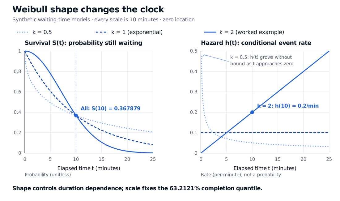
For $k<1$ , both density and hazard grow without bound as $t\downarrow0$ . The density spike is integrable: it creates no probability atom at zero. At $k=1$ the density's right limit is $1/\eta$ ; at $k>1$ it is zero. An ordinary Weibull hazard is monotone, so it cannot represent a hazard that first falls and then rises.

A ten-minute scale is not a ten-minute average

Suppose an operations team uses a hypothetical model for the time until an unresolved trade reconciliation is completed, measured from when it enters a particular workflow:

k=2,\qquad \eta=10\text{ minutes}.

This is a stipulated teaching model, not a calibration to operational records. It gives

S(t)=e^{-(t/10)^2},\qquad h(t)=\frac{2}{10}\frac{t}{10}\text{ min}^{-1},

where $t$ in the numerical expression is elapsed minutes. The model's increasing completion hazard says older unresolved cases have a greater immediate chance of completion, which could be a hypothesis about an escalation process. It does not say the hypothesis is true.

Question	Result
Probability still unresolved after ten minutes	$S(10)=e^{-1}\approx0.367879$ , or 36.7879%
Time by which half are completed	$10\sqrt{\ln 2}\approx8.325546$ minutes
Expected completion time	$5\sqrt{\pi}\approx8.862269$ minutes
Variance of completion time	$100(1-\pi/4)\approx21.460184\text{ min}^2$
Hazard at ten minutes	$0.2\text{ min}^{-1}$

For every positive shape,

S(\eta)=e^{-1}

. Thus scale is the time by which approximately 63.2121% of cases are completed, not generally the mean or median. Nor is it an arrival intensity: ten minutes is a duration, while intensity is measured per minute.

Weibull survival and hazard curves for shapes 0.5, 1 and 2, all with scale ten minutes. All survival curves pass through 0.367879 at ten minutes; the shape-two hazard there is 0.2 per minute. The shape-0.5 hazard diverges near zero.

Original synthetic comparison with zero location. Changing shape changes duration dependence while preserving the survival probability at the shared scale. The horizontal window ends at 25 minutes; the distributions continue beyond it.

Waiting changes the next question

Once a reconciliation is still unresolved after ten minutes, the relevant conditional probability of completing in the next five minutes is

\begin{aligned} \mathbb{P}(10<T\le15\mid T>10) &=1-\frac{S(15)}{S(10)}\\ &=1-e^{-1.25}\approx0.713495. \end{aligned}

That is 71.3495%, compared with 22.1199% for completion during the first five minutes of a fresh case,

F(5)=1-e^{-0.25}

. Restarting the clock at ten minutes and applying the original five-minute CDF would discard the model's increasing hazard. Only shape one has the exponential memoryless property.

This conditioning uses only the fact that the case is unresolved. If new information reveals its size, complexity or workflow stage, a single unconditional Weibull model need not describe the revised outlook. If observation ends before completion, the elapsed duration is a censored observation, not an observed completion time.

Quantiles, moments and simulation

Solving

F(t)=p

gives the quantile function:

Q(p)=\eta[-\ln(1-p)]^{1/k},\qquad0<p<1.

In particular, the median is $\eta(\ln2)^{1/k}$ . The general moments are

\begin{aligned} \mathbb{E}[T]&=\eta\Gamma\left(1+\frac1k\right),\\ \text{Var}(T)&=\eta^2\left[\Gamma\left(1+\frac2k\right)-\Gamma\left(1+\frac1k\right)^2\right]. \end{aligned}

Here

\Gamma(a)=\int_0^\infty u^{a-1}e^{-u}\,du

is the Gamma function; it is distinct from the Gamma distribution. All positive-order moments exist for positive shape and scale.

A useful construction explains the family: if

E

is exponential with rate one, then

T=\eta E^{1/k}

is Weibull. Equivalently, inverse transform sampling uses

T=Q(U)

for a uniform draw

U

(0,1)

. The Random Number Generation lesson develops inversion and the unit-scale Weibull recipe; its full content requires membership and has a public preview. Generating independent draws creates an independent-duration model because of the sampling construction, not because the family name guarantees independence.

Keep the event and parameterisation explicit

Some references use $S(t)=e^{-\lambda t^k}$ . This is the same unshifted family with $\lambda=\eta^{-k}$ ; $\lambda$ has units of time to the power $-k$ and is a constant hazard only when $k=1$ . Other implementations add a location parameter, which changes the earliest possible event time. Record the actual survival formula alongside parameter estimates.

In credit applications, reduced-form default models connect hazard to default survival and distinguish physical probabilities from pricing probabilities. That full lesson requires membership and has a public preview. An operational completion model and a risk-neutral default model need different data, event definitions and interpretations even when their algebra matches.

A further financial use is duration-based backtesting of Value at Risk. Christoffersen and Pelletier use a Weibull alternative to an exponential no-hit-duration benchmark. A shape below one gives a decreasing hazard, accommodating excess very short and very long durations associated with violation clustering. This concerns the event process implied by durations; a Weibull marginal alone does not establish serial dependence between successive duration observations. Daily hit durations are discrete, so a continuous-duration approximation and its test calibration need care.

Finally, the bounded reverse-Weibull extreme-value family encountered in block-maxima theory is a different parameterisation and use of the name. The ordinary waiting-time Weibull defined here has no finite upper endpoint.

Sources

Joseph K. Blitzstein and Jessica Hwang, Introduction to Probability, second edition (CRC Press, 2019), Example 6.5.5 and warning 6.5.6: exponential-power construction, memorylessness and parameter conventions.
NIST/SEMATECH, e-Handbook of Statistical Methods, §8.1.6.2, “Weibull”: two-parameter lifetime model, survival, hazard and moments.
NIST/SEMATECH, §1.3.6.6.8, “Weibull Distribution”: density, inverse distribution and support.
Peter Christoffersen and Denis Pelletier, Backtesting Value-at-Risk: A Duration-Based Approach, author manuscript dated 24 October 2003, §3, equations (8)–(10); published in Journal of Financial Econometrics 2 (2004), 84–108.

Start with the survival curve

A ten-minute scale is not a ten-minute average

Waiting changes the next question

Quantiles, moments and simulation

Keep the event and parameterisation explicit

Sources

Related terms

Conditional probability

Continuous random variable

Cumulative distribution function

Expected value

Exponential distribution

Gamma distribution

Probability density function

Quantile function

Survival function

Value at risk

Variance