Define the target, sampling frame and model before estimating trading costs; distinguish mean from median and standard error from justified uncertainty intervals.
Statistical estimation
Statistical estimation is the process of using observed data to infer an unknown feature of a population or data-generating process, together with an assessment of uncertainty. The target might be an expected execution cost, a default probability, a return covariance matrix or an entire distribution. An estimate is useful only when its target and the conditions connecting the observations to that target are clear.
For a trading desk, the difficult question often comes before the calculation: are we estimating the cost of a typical trade, the expected cost per trade, or the cost per unit of traded notional? Those questions can produce different answers from the same records.
Define the target before choosing the formula
The estimand is the quantity we want to learn. A population mean, for example, is a feature of a specified distribution. The estimator is the rule applied to a random sample; the estimate is its realised output after the data arrive:
θ^=T(X1,…,Xn),θ^obs=T(x1,…,xn).
Here θ denotes the unknown target. In frequentist analysis it is fixed; the estimator varies across possible samples. Estimation includes point estimation, which returns a single value, and interval estimation, which uses a procedure to express uncertainty around the target.
A workable estimation specification answers four questions:
Decision
Execution-cost example
What is the target?
Expected adverse slippage, in basis points, per eligible trade under a specified execution policy.
Which observations represent it?
Define instruments, venues, order sizes, trading hours and dates; retain costly trades as well as cheap ones.
What information was available?
Fix the price benchmark and timestamp rule; use only information available when evaluating the policy.
Which assumptions support inference?
Specify dependence, changing market conditions and any distributional model before interpreting uncertainty.
The sampling frame is the set of eligible observations from which records can be collected. If failed orders or stressed sessions are excluded, a precise estimate from the retained trades can still answer the wrong question. More observations do not automatically repair selection bias.
Five trades: mean cost or middle cost?
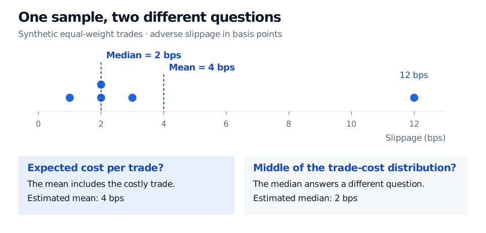
Consider synthetic per-trade adverse slippages of 1, 2, 2, 3 and 12 bps, measured against a consistently defined decision-price benchmark. Positive means worse execution. Give each trade equal weight. The target is the expected cost of a trade drawn from the same specified trade-generating process, not a notional-weighted cost.
The sample mean is
xˉ=51+2+2+3+12=4 bps.
The sample median is the middle ordered observation: 2 bps. It estimates the population median, a different target. It is less sensitive to the large observation, but that does not make it a more accurate estimate of the population mean. A genuine expensive trade belongs in an expected-cost calculation; treating it as an error requires evidence about the record, not discomfort with its size.
Five synthetic trade costs of 1, 2, 2, 3 and 12 bps. The mean is 4 bps and the median is 2 bps; they estimate different population characteristics.
Original synthetic equal-weight example. Dots are observed trade costs, not an estimated sampling distribution. Mean and median answer different questions.
The 12 bps observation raises the mean from the other four trades' mean of 2 bps to 4 bps. That is an influence diagnostic, not a reason to discard it. If the desk wants cost per unit of notional, it needs the trade notionals and an explicitly weighted calculation; these five costs alone do not determine that answer.
Add uncertainty without pretending to know more
For illustration, assume independent and identically distributed trade costs with a finite population variance. The mean estimator then has variance σ2/n. Using the sample variance with divisor n−1 gives
The plug-in estimate of the mean's standard error is therefore
SE(Xˉ)=5s=520.5≈2.02485 bps.
This estimates how much the sample mean would vary across repeated samples under the assumptions. It is neither the dispersion of individual trades nor a guaranteed bound on estimation error. Although s2 is unbiased for the population variance under these assumptions, taking its square root does not generally produce an unbiased standard-error estimator.
A standard error is also not yet a confidence interval. An exact Student-t interval for the mean requires an independent normal sample; an approximate normal interval needs a defensible sampling approximation. Five observations with a prominent upper-tail value do not establish either justification. The confidence interval procedure must be chosen with the sampling model, not attached mechanically to the output. The NIST discussion of confidence limits explains the repeated-sampling interpretation of coverage.
Trades within one parent order or market episode may be dependent. In general,
Var(Xˉ)=n21(i=1∑nVar(Xi)+2i<j∑Cov(Xi,Xj)).
The simple s/n calculation omits those covariance terms. Dependence may call for cluster-aware inference or a time-series method, provided enough independent groups or time history exist. Resampling five records cannot manufacture missing market regimes or reveal an unseen tail.
Validate the connection to the decision
Estimators can be compared by bias, variance, mean squared error and stability, relative to the same target and assumptions. Maximum likelihood estimation selects parameters by their fit to the observed data under a specified probability model; it does not verify that the model represents future trades. For the bias, risk and likelihood derivations behind these comparisons, Estimation and Maximum Likelihood provides a public preview; the full lesson requires membership.
For the desk, validation means checking benchmark timestamps, missing records and units; examining sensitivity to costly trades and market periods; and comparing subsequent realised costs with the frozen estimate. A later sample tests transport to another period, while sampling uncertainty describes variation under the assumed process. A market-regime change can defeat that transport even if the original estimator was calculated correctly.
A useful report therefore says: what was estimated, from which eligible records, under which policy and assumptions, with which uncertainty assessment, and with what validation evidence. “Average slippage: 4 bps” leaves most of the estimation problem unanswered.
Sources
Larry Wasserman, All of Statistics: A Concise Course in Statistical Inference (Springer, 2004), §6.2 on models and functionals; §6.3.1 on point estimation, bias, consistency, standard errors and mean squared error.