Interval estimation: Definition & Examples

Interval estimation uses sample data to estimate an unknown parameter with a range of values, together with a stated rule for interpreting the uncertainty. A point estimate of a strategy's mean daily excess return might be 0.4%. An interval estimate also tells the researcher how imprecisely the experiment has pinned down that mean.

The range alone is incomplete. You need to know what is being estimated, how the endpoints were constructed, and what the probability statement means. A frequentist confidence interval and a Bayesian credible interval can both estimate a parameter, but their interpretations differ.

Endpoints are an estimation rule

Write an interval estimator for a scalar parameter $\theta$ as

C(X)=[L(X),U(X)],

where $X$ denotes the sample and the lower and upper endpoints are functions of it. Before sampling, the endpoints vary with the data. After observing $X=x$ , the reported interval $[L(x),U(x)]$ is fixed.

For a frequentist procedure with confidence level $1-\alpha$ , the usual coverage requirement is

\mathbb{P}_{\theta}\!\left(L(X)\le\theta\le U(X)\right)\ge 1-\alpha \quad\text{for every admissible }\theta.

The probability describes repeated samples generated under the model, with the true parameter held fixed. Some procedures have exactly the target coverage; others are conservative, and large-sample procedures may only approach it as the sample grows. Simply placing “95%” beside two numbers does not establish any of these properties. Casella and Berger's §9.1 makes this distinction between a random interval and its realised endpoints; NIST explains the repeated-sampling interpretation.

Nor must every interval look like an estimate plus or minus a symmetric margin. A one-sided bound may be more appropriate for a predeclared question, while skewed sampling distributions can produce unequal distances from the estimate to the endpoints.

A return estimate with visible uncertainty

Consider an original, deliberately simplified research experiment. A strategy is fixed before data collection. Its 100 daily excess returns, after a specified fixed cost deduction, are assumed independent and identically distributed under a normal model, with unknown mean

\mu

and known population standard deviation of 2 percentage points. The observed sample mean is 0.4 percentage points, meaning a 0.4% daily excess return. All calculations below use percentage points, abbreviated pp.

Known volatility is an assumption of this teaching experiment, not something a historical sample makes certain. Under that assumption, the mean's standard error is

\operatorname{SE}(\bar X)=\frac{\sigma}{\sqrt n} =\frac{2}{\sqrt{100}}=0.2\text{ pp}.

Because $Z=(\bar X-\mu)/(\sigma/\sqrt n)$ is standard normal, taking the central 95% of its distribution and rearranging gives

\begin{aligned} C(X)&=\left[\bar X-z_{0.975}\frac{\sigma}{\sqrt n},\; \bar X+z_{0.975}\frac{\sigma}{\sqrt n}\right],\\ z_{0.975}&\approx1.9599639845. \end{aligned}

This procedure has exactly 95% coverage under the stated model. Its observed result is

0.4\pm1.9599639845(0.2) \approx[0.0080,\;0.7920]\text{ pp}.

The unrounded endpoints are approximately 0.0080072 and 0.7919928 pp. The interval is just above zero, but that does not establish a persistent tradable edge. Even the model-based estimate allows a mean very close to zero; changing costs, strategy selection or a changing return distribution can matter more than the last decimal place.

NIST's known-standard-deviation construction gives this normal interval. If the population standard deviation is instead estimated by the sample standard deviation

S

, the exact IID-normal construction uses the Student

t

critical value with

n-1

degrees of freedom and standard error

S/\sqrt n

. Substituting an estimated volatility into the known-volatility formula does not retain its exact finite-sample justification.

Estimating the mean does not contain the next return

The 95% interval above estimates the population mean. It does not say that 95% of daily returns fall between its endpoints.

For one independent future return from the same normal population, a prediction interval must also account for that return's own variability. In this known-volatility experiment,

\text{Var}(X_{n+1}-\bar X)=\sigma^2+\frac{\sigma^2}{n},

so an exact 95% prediction procedure is

\bar X\pm z_{0.975}\sigma\sqrt{1+\frac1n}.

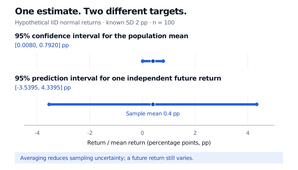
With the same data it produces approximately [−3.5395, 4.3395] pp. Its coverage is over the original sample and the independent future observation together. It is much wider because averaging reduces uncertainty about the mean without removing variability from the next outcome. NIST's prediction-limits documentation develops the corresponding estimated-volatility construction.

Hypothetical IID normal returns with known population SD 2 pp, sample size 100 and sample mean 0.4 pp. On one common scale, the exact 95% confidence interval for the mean is [0.0080, 0.7920] pp, while the exact 95% prediction interval for one independent future return is [−3.5395, 4.3395] pp.

Original model illustration. Both intervals use the same sample mean and known population volatility; their targets differ. Filled endpoints are included. Neither is a guarantee about future markets.

Reading the interval in a research report

A frequentist 95% confidence level is not a posterior probability of 95% that the fixed mean lies inside these particular observed endpoints. A Bayesian 95% credible interval instead contains 95% of the parameter's posterior probability, conditional on the observed data, likelihood and prior. Its repeated-sampling coverage need not equal 95%. The intervals may sometimes coincide numerically without making their interpretations interchangeable.

Width also needs context. With this same known-volatility method and fixed sample size, raising the confidence level widens the interval. At a fixed confidence level and population volatility, quadrupling the sample size halves its width. These comparisons assume the same sampling design and stable population; collecting more observations from a changed regime does not necessarily provide more information about the mean you originally wanted.

For financial data, check autocorrelation, overlapping holding periods, changing volatility and how the strategy was selected. They can undermine the simple IID calculation. Approximate intervals based on robust sampling variances or a suitably chosen bootstrap need their own assumptions. Narrow error bars do not repair biased data or a misspecified model, and nominal coverage for one prespecified strategy does not automatically survive a search over many strategies.

For the normal-family derivation and the connection between intervals and tests, continue with Confidence Intervals and Hypothesis Testing. The public page offers a preview; the full lesson requires membership.

Sources

George Casella and Roger L. Berger, Statistical Inference, 2nd ed., §9.1 (interval estimators and coverage), §9.2.2 (pivotal quantities), and §9.2.4 (Bayesian intervals).
NIST/SEMATECH, §7.1.4: What are confidence intervals? — known-population-standard-deviation normal interval and one-sided versus two-sided intervals.
NIST/SEMATECH, §1.3.5.2: Confidence Limits for the Mean — coverage interpretation and the normal-family interval when the standard deviation is estimated.
NIST Dataplot: Prediction Limits — prediction of one or more new independent observations, distinguished from parameter estimation.

Endpoints are an estimation rule

A return estimate with visible uncertainty

Estimating the mean does not contain the next return

Reading the interval in a research report

Sources

Related terms

Confidence interval

Normal distribution

Point estimation

Standard error