Distinguish a parameter, an estimator and its observed point estimate using three rejected orders out of twenty, then interpret sampling uncertainty.
Point estimation
Point estimation uses sample data to report one value for an unknown quantity. In a statistical model, that quantity is a parameter; the calculation rule is an estimator, and its value for the observed data is a point estimate. A single reported number is useful for making a calculation. It does not reveal how accurately the quantity has been measured.
Three rejected orders out of twenty
An execution team audits a prespecified set of 20 submitted orders routed under the same conditions. Three were rejected. For this hypothetical example, suppose each order has the same unknown rejection probability p, and the rejection indicators are independent Bernoulli observations. Define Xi=1 for a rejection and Xi=0 otherwise, and let K be the total number of rejections.
Object
Meaning in the audit
Parameter p
Unknown rejection probability under the stipulated routing conditions
Estimator p^=K/20
Rule: divide the rejection count by the number of audited orders
Point estimate p^=3/20=0.15
Observed rejection rate: 15%
Uncertainty interval
A range produced by a specified inference method, rather than another name for 15%
The estimate can be entered into an execution-cost model as a provisional input. It is not a known true probability, nor does it guarantee anything about the next order. Under the model, the next rejection is still a binary outcome with unknown probability p. Substituting 0.15 provides an estimated probability, not a guarantee.
The target matters before the arithmetic. A rate for this router and these conditions need not estimate the rate during a venue outage, for another order type, or after a routing-policy change. Including only acknowledged orders would also omit precisely the rejected submissions being counted.
What changes across samples?
Before the audit, K is random. The rule stays fixed, but another set of 20 orders could produce a different estimate. Under the stated model, K has a binomial distribution, giving
E[p^]=p,Var(p^)=20p(1−p).
The expectation follows because each indicator has mean p; the variance follows by adding the variances of the independent indicators and dividing by 202. Thus the estimator is unbiased: its repeated-sample average equals p. That property does not say that this sample's estimate equals p.
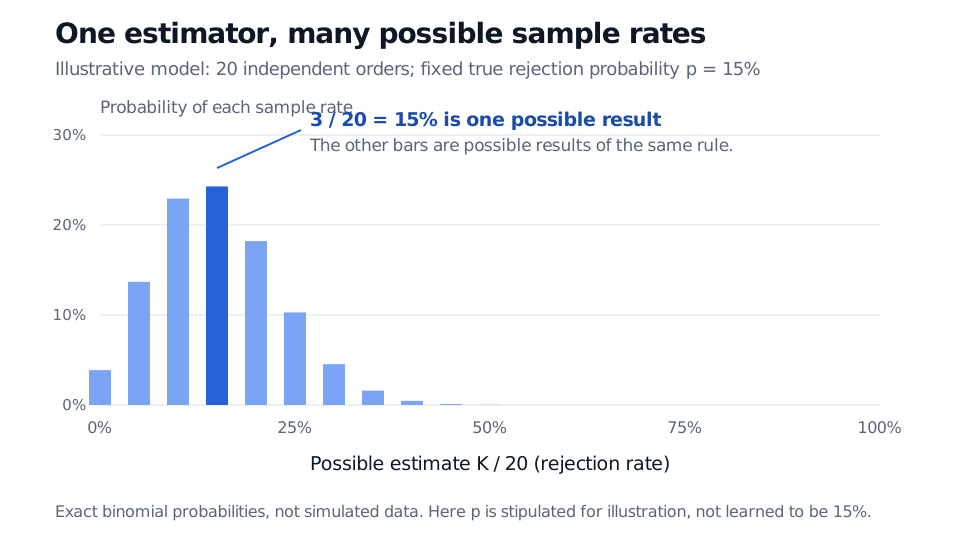
Exact sampling distribution of K divided by 20 for 20 independent Bernoulli orders with stipulated true rejection probability 15%. Possible estimates occur in steps of five percentage points; the 15% estimate is highlighted among many possible outcomes.
Original exact sampling distribution under an illustrative fixed p=0.15. The stipulated truth makes the spread visible; observing three rejections does not establish that this is the true distribution.
The standard error is the estimator's standard deviation. Here it depends on the unknown p. Replacing p by 0.15 gives an estimated standard error
SE(p^)=200.15(1−0.15)≈0.0798,
or about 7.98 percentage points. That is a measure of sampling spread, not a confidence level or a bound on the estimation error. With only three rejections, a symmetric normal interval can be unreliable; an interval should come with a method and assumptions. A confidence interval adds a repeated-sampling coverage statement, rather than turning the point estimate into certainty. If no rejections were observed, the same plug-in standard error would be zero; this would not prove that rejection is impossible.
Choosing and using the number
Point estimation names the task, not one universal calculation. Maximum likelihood estimation is one way to choose an estimator; for this Bernoulli model it gives the observed rejection rate. Other methods can produce different estimates, and their merits depend on the target, assumptions and consequences of error.
For a useful report, state the estimate together with the sample size, sampling window, order-selection rule and uncertainty method. More observations reduce the variance above when the common-probability independence model holds. They do not repair a biased selection process or make a changing router behave like a stable one.
For a fuller derivation, Estimation and Maximum Likelihood develops estimator risk, Bernoulli likelihood and the limitations of large-sample standard errors. The public page is a preview; the complete lesson requires membership.
Sources
Larry Wasserman, All of Statistics: A Concise Course in Statistical Inference (Springer, 2004), §6.3.1, especially Example 6.8: point estimation, Bernoulli sample proportions and estimated standard errors.
Hyebin Song, Penn State STAT 415 (Spring 2021), Point Estimation: statistical model, bias and mean squared error.