A test for departures in either direction: calculate both normal tails, separate a negative significant result from a positive edge, and read the matching confidence interval.
Two-sided test
A two-sided test is a hypothesis test whose alternative allows departures from a specified parameter value in either direction. For a mean return, it asks whether the mean differs from a benchmark, rather than specifically whether it exceeds that benchmark.
That distinction matters when reviewing a strategy. A statistically detectable negative mean can reject “zero expected excess return” while providing no evidence for the positive edge the researcher hoped to find.
The question determines the tails
Let μ be the strategy's mean daily excess return after specified costs and relative to a specified cash benchmark. Consider
H0:μ=0,H1:μ=0.
Both negative and positive means belong to the alternative hypothesis. In the symmetric normal-mean test below, departures of equal standardized magnitude count as equally extreme. A 5% significance level is divided into two rejection tails of 2.5% each. It is a total error allowance, not 5% per tail.
Fix the hypotheses, sample window and decision rule before looking at the data. A one-sided test chosen because the observed average happens to be positive or negative is a different procedure from one whose direction was fixed in advance.
A negative result can be significant
Consider a hypothetical sample of 64 daily excess returns. Stipulate independent, identically distributed normal observations with a known population standard deviation of 1 percentage point (pp). The observed sample mean is −0.25 pp per day. These assumptions make the calculation exact; they are not claims about real return data.
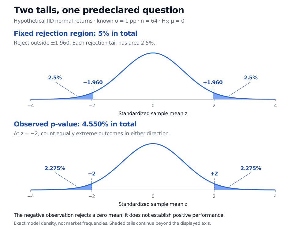
Each observed tail contributes about 2.275%, for a total of 4.550%. The positive tail is counted even though the observed result is negative: the predeclared alternative regards either direction as evidence against zero.
The 5% rule rejects when
∣zobs∣>Φ−1(0.975)≈1.95996,
equivalently when p<0.05. Here it rejects. The critical values are fixed by the chosen level; the p-value uses the observed magnitude. They need not delimit the same tail area.
Two standard normal panels: the fixed rejection tails beyond ±1.960 each have area 2.5%; the observed p-value tails beyond ±2 each have area 2.275%, totaling 4.550%.
Original exact normal-model calculation for the hypothetical sample. The first panel shows the fixed 5% rejection region; the second shows the observed p-value. Shaded tails extend beyond the displayed axis.
Keep the sign in the report
“Significant” alone loses the economic meaning. The estimated mean is negative. Its matching 95% confidence interval is
xˉ±Φ−1(0.975)nσ=−0.25±1.95996398(0.125)≈[−0.49500,−0.00500] pp per day.
Zero falls outside the interval, agreeing with the test. The interval also shows how close the upper endpoint is to zero. Its 95% coverage describes repeated sampling under the model, not a posterior probability assigned to this realized interval. With strict rejection and a closed interval, a null value exactly at an endpoint is not rejected.
For the explicitly positive alternative μ>0, this same negative observation would instead have right-tailed p-value 1−Φ(−2)≈0.97724987. Evidence against zero in either direction is therefore not a positive-edge certificate. Nor does it establish that a negative edge will persist, justify reversing the strategy, or show that the effect survives execution costs and a search across many strategies.
The known-volatility assumption also matters. When the population standard deviation is estimated from this normal sample, the usual exact mean test uses Student's t distribution with n−1 degrees of freedom. Confidence Intervals and Hypothesis Testing derives that change and the matching interval (public preview; full lesson requires membership). Dependent returns require an appropriate sampling-variance treatment; adding a second tail does not repair an invalid standard error.
What “two-sided” does not settle
Doubling one tail works here because the normal reference law is symmetric and extremeness is defined by absolute standardized distance. It is not a universal definition for asymmetric or discrete tests: specify the test's ordering of outcomes and its two-sided p-value convention.
Finally, failure to reject equality does not establish practical equivalence. A noisy estimate can be compatible with zero and with economically large positive or negative means. Demonstrating that an effect lies within a tolerable range requires a separately designed equivalence analysis.
John A. Rice, Mathematical Statistics and Data Analysis, 3rd ed., Duxbury, 2007, §§9.2.1–9.2.3 and 9.3. P-values, directional alternatives, and inversion of normal-mean tests to obtain confidence intervals.