A significance level bounds false rejection under the null. Compare exact normal size with a conservative binomial test and see why a 5% rule does not cover an entire strategy search.
Significance level
The significance level, written α, is a chosen upper bound on the probability that a hypothesis test rejects its null hypothesis when that null is true. It sets a false-alarm constraint for the testing procedure before the data are examined.
A quant researcher might choose a 5% level for a prespecified test of a strategy's mean return. That choice controls a particular statistical error under a stated model. It does not make a significant strategy 95% likely to be profitable, or guarantee that only 5% of the strategies selected by a research team are false discoveries.
The target and the attained rate
Let R be the test's rejection region, and let Θ0 contain every parameter value allowed by the null. A level-α test satisfies
θ∈Θ0supPθ(X∈R)≤α.
Rejecting a true null is a Type I error. The supremum is the largest false-rejection probability across the null models, or its limiting upper value if no maximum is attained. It matters when the null is composite: controlling the error at one convenient parameter value is insufficient unless it also controls the others.
The size of the test is that supremum. Here, “level” refers to the allowed bound and “size” to the attained value; some sources use the words interchangeably. A test with size 4% is a level-5% test, even though it does not use the entire allowance.
Two designs with a 5% allowance
A continuous statistic can hit the target exactly. Suppose independent normal returns have a known, positive population standard deviation σ. For a fixed sample of size n, test H0:μ=0 against H1:μ=0 using
Z=σ/nXˉ.
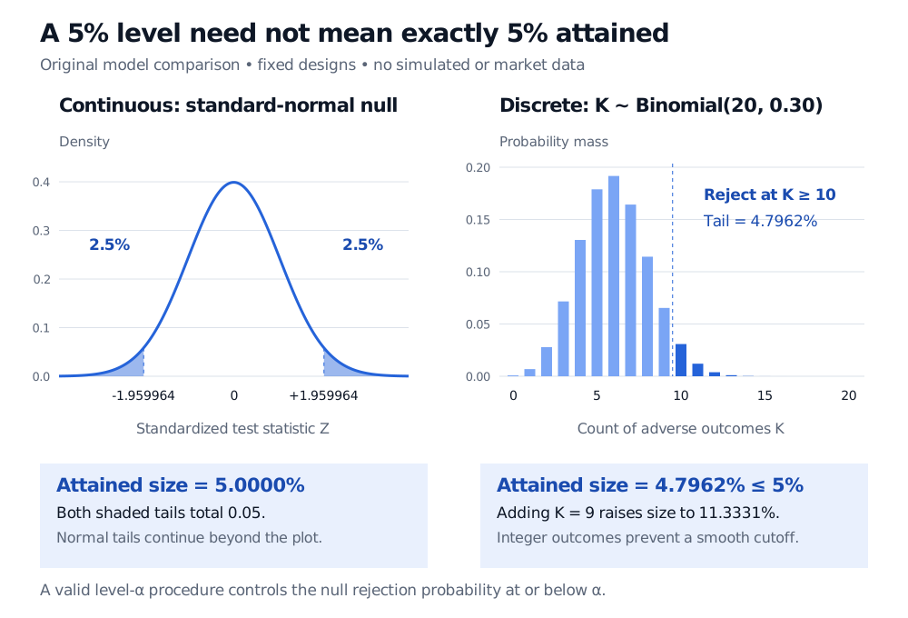
Under this null, Z has a standard normal distribution. With the exact critical value c=Φ−1(0.975)≈1.959964, reject when ∣Z∣>c. Each tail has probability 2.5%, so the size is exactly 5%. The exact statement uses the quantile, rather than the rounded decimal cutoff. Because this distribution is continuous, including the endpoints would not change the probability.
Known volatility is an assumption of this example. Estimating volatility from the same normal sample leads to a Student t reference distribution and different critical values. Real return dependence can require a different sampling-uncertainty calculation altogether.
An integer count may leave some allowance unused. Consider a hypothetical execution check on 20 independent orders. Each order has the same probability p of an adverse outcome. Test H0:p≤0.30 against H1:p>0.30, using the adverse-outcome count K.
At the null boundary, K follows a binomial distribution with parameters 20 and 0.30. For the rule “reject when K≥10,”
This is the worst case over p≤0.30: increasing p makes high counts more likely. The test therefore has level 5% and size approximately 4.7962%. Lowering the cutoff to 9 makes the size approximately 11.3331%, exceeding the allowance. The missing fraction is a consequence of discrete probability mass, not an inaccurate normal approximation; these are exact binomial calculations. Randomized boundary decisions can fill such a gap in statistical theory, but the stated execution rule is deterministic.
Under a standard-normal null, rejection outside minus and plus 1.959964 has total probability 5%, split equally between tails. For 20 independent Bernoulli outcomes at p 0.30, rejecting at K at least 10 has size 4.7962%; including K equals 9 raises size to 11.3331%.
Original comparison of two fixed model-based designs. The left panel shades the exact normal rejection tails; the right shows every possible binomial count, with the rejection outcomes in dark blue. Neither panel uses market data.
Choosing a level is a research-design decision
A smaller α makes false rejection harder, but generally reduces statistical power when the sample size and test family stay fixed. The consequence of a missed real effect matters alongside the consequence of a false alarm. There is no mathematical rule making 5% suitable for every trading, model-validation or execution decision.
Specify the null, alternative, statistic, direction, sampling window and stopping rule along with the level. Changing from 5% to 10% after seeing an inconvenient result changes the procedure whose error probability was promised. Choosing the favorable tail after observing the sign creates the same problem.
The observed p-value is a separate quantity. The level is a design threshold; the p-value is computed from the data and null reference model. For a valid p-value, the rule “reject if P≤α” controls the false-rejection probability at or below α. With discrete tests, attained probabilities can jump as the threshold changes.
For a fuller derivation of normal-sample tests and their matching intervals, Confidence Intervals and Hypothesis Testing connects the critical region to a confidence interval. The full lesson requires membership; its preview is public.
One test's allowance does not cover a strategy search
Suppose 20 tests have true nulls, are independent, and each has size exactly 5%. Then the probability of at least one false rejection is
1−(1−0.05)20≈0.641514,
or 64.15%. The expected number of false rejections is 1. Neither number is the proportion of reported discoveries that must be false. Independence is needed for this particular probability calculation; correlated strategy tests require a different calculation.
Multiple hypothesis testing addresses error across a family of tests. Repeated monitoring also needs a procedure designed for its stopping rule. A per-test level does not automatically cover either search or repeated looks.
Finally, the bound depends on the sampling model being appropriate. A nominal 5% label cannot repair dependent orders treated as independent, underestimated return uncertainty, or a null chosen after inspecting the results. Report the effect estimate and its uncertainty, the design and the search performed. Statistical significance alone does not establish economic value after costs.
Sources
George Casella and Roger L. Berger, Statistical Inference, 2nd edition (2002), §8.3.1, Definitions 8.3.5–8.3.6 — distinction between size and level, and control across a composite null.
John A. Rice, Mathematical Statistics and Data Analysis, 3rd edition (2007), §9.2.1 — specifying the level before analysis and interpreting p-values.