A Type I error is the rejection of a true null hypothesis. It is also called a false positive. For example, a test may flag a strategy's mean excess return as different from zero even though its true mean excess return is zero. The error concerns the statistical claim being tested; a significant result alone does not establish a profitable trading strategy.
The NIST definition ties the error to both a decision and the truth of the null. A large loss, a bad forecast or a failed strategy is not automatically a Type I error. First identify which null was rejected.
The error is an event; the level is a design choice
A hypothesis test specifies a rejection region before the data are evaluated. If the parameter is , its false-rejection probability at a particular true-null value is
where is the set of parameter values allowed by the null. A test has level when
The supremum is its size: the worst-case false-rejection probability over the null. Thus a test with level 5% need not reject exactly 5% of the time at every null value. Discrete tests, for example, can be conservative. Casella and Berger distinguish a size- test, whose supremum equals , from a level- test, whose supremum is at most .
The probability describes repetitions of the specified procedure under the null model. It is not the probability that this particular rejected null is true. Nor does it mean that 5% of all reported discoveries must be false. Those questions require information beyond the test's level, including which claims are true and how often the procedure detects alternatives.
Where the 5% goes
Consider a fixed, two-sided test of against for a strategy's mean daily excess return. Stipulate independent, identically distributed normal returns, a fixed sample size , and a genuinely known population standard deviation . These are teaching assumptions, not properties asserted about market data.
Under the null, the standardised mean is
Let , where is the standard normal cumulative distribution function. Reject when . Then
Each rejection tail has probability 2.5%. Because the reference distribution is continuous, including the boundary would not change this probability. Here the test has exact size 5%: even a correctly calibrated procedure sometimes rejects a true null.
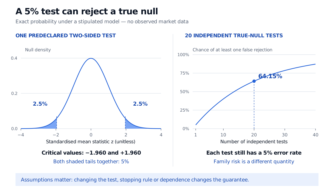
Original exact-model calculation. Left: one predeclared two-sided normal test. Right: all nulls are true and rejection events are independent; the marker shows 20 tests. No market observations or simulation are used.
If the standard deviation is estimated, the normal cutoff is not automatically exact; under iid normal sampling the corresponding mean test uses a Student reference distribution. Serial dependence, selecting the sample window after seeing returns, or repeatedly checking until significance also changes the procedure. A nominal 5% label cannot repair an incorrectly calibrated test. The Confidence Intervals and Hypothesis Testing lesson develops these sampling-model distinctions; its public preview is open, while the full lesson requires membership.
One false discovery from a search
Now suppose a researcher tests 20 different strategy claims. All 20 nulls are true, every test has false-rejection probability 5%, and their rejection events are independent. The probability of no false rejection is . Therefore,
That is 64.15%, despite the 5% rate for each individual test. The expected number of false rejections is ; it is not a promise of exactly one in a particular search. This expectation does not require independence, whereas the product formula above does. Perfectly identical rejection events would instead give a 5% chance of at least one rejection.
This distinction matters when only the winning backtest is reported. The search creates more chances to reject a true null. Correlated strategies require a dependence-aware analysis; counting them as independent without justification does not establish a valid family error rate.
One remedy for a defined family is the Bonferroni rule: test each claim at level . The union bound then limits the probability of any false rejection to at most 5%, without requiring independence. It presupposes valid individual tests and an adequately specified family; it does not fix leakage or unreported additional searches. Rice's discussion of fishing expeditions and NIST's Bonferroni guide explain the simultaneous-error logic.
Reducing the rejection region generally sacrifices statistical power against a fixed alternative in a fixed design. A Type II error is the other mistake: failing to reject when the null is false. Choosing an error tolerance therefore belongs with the research question, sample design and consequences of each decision, before inspecting the result.
Sources
- NIST, Type I Error: definition of a false rejection.
- NIST/SEMATECH, Quantitative Techniques, §1.3.5: rejection regions, significance levels and power.
- NIST/SEMATECH, Bonferroni's Method, §7.4.7.3: simultaneous error control via the Bonferroni inequality.
- John A. Rice, Mathematical Statistics and Data Analysis, 3rd edition, Duxbury, 2007, §9.2 and §11.4.8: testing errors and fishing expeditions.
- George Casella and Roger L. Berger, Statistical Inference, 2nd edition, Duxbury, 2002, §8.3.1, Definitions 8.3.5–8.3.6: distinction between test size and level.