Why a test can miss a real trading effect: calculate Type II error under a specified alternative and see how sample size and significance thresholds change it.
Type II error
A Type II error occurs when a hypothesis test fails to reject a false null hypothesis. A strategy can have a real positive expected excess return and still produce a history that does not cross the test's rejection threshold. The test has missed an effect; the effect has not disappeared.
The probability of this error is usually written β. It must be evaluated at a specified alternative hypothesis: a small edge is generally harder to detect than a large one. If R is the rejection region and the true parameter is θ∈/Θ0, then
β(θ)=Pθ(X∈/R),Power(θ)=1−β(θ).
Here X denotes the full random sample. Statistical power is the probability of detecting that particular departure from the null. Neither quantity is the probability that the null is true after seeing the data.
The same threshold can miss a real edge
Consider an illustrative strategy with independent, identically distributed normal excess returns measured in percentage points per period, with known population standard deviation σ=2. Take a fixed sample of n=100 periods and prespecify the two-sided test
H0:μ=0,H1:μ=0,α=0.05.
This choice detects departures in either direction. It does not specifically test whether a strategy is profitable. The standard error of the sample mean is se=σ/n=0.2 percentage points. With z0.975≈1.959964, reject when
∣Xˉ∣>c,c=z0.975se≈0.391993.
Use the unrounded cutoff for calculations. The non-rejection interval is [−c,c]; equality does not trigger rejection. Because this model is continuous, the endpoints have probability zero.
Now suppose the true mean is μ1=0.5 percentage points per period. This deliberately large synthetic effect makes the mechanism visible; it is not a calibrated return forecast. Under that alternative, Xˉ∼N(0.5,0.22). Writing Φ for the standard normal cumulative distribution function,
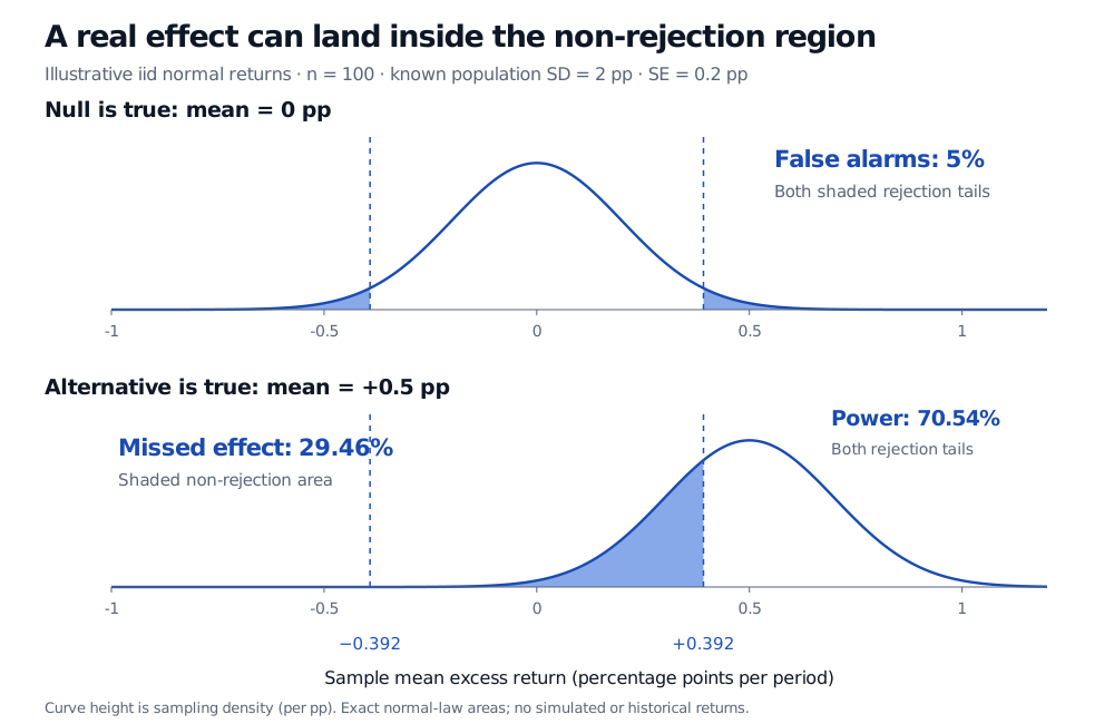
The test misses this real mean in 29.46% of repeated samples from the stipulated model. Its power is 70.54%. Both rejection tails count toward power, even though the true mean is positive; the negative-tail contribution is tiny but included.
Two sampling distributions with identical cutoffs at minus and plus 0.392 percentage points: under mean zero, rejection tails total 5%; under true mean plus 0.5 percentage points, the shaded non-rejection area is beta 29.46% and power is 70.54%.
Original normal-model calculation, with n = 100 and known population SD = 2 percentage points. The cutoff stays fixed while the sampling distribution changes. Curves are shown over a finite axis range; reported areas use the full normal law.
The upper panel's 5% describes Type I error, a false rejection when the null is true. It places no 5% ceiling on the lower panel's missed-effect probability. The probabilities concern different states of the world.
What changes the miss rate?
Keep the true mean at 0.5 and population SD at 2 percentage points. For this same two-sided normal test:
Independent observations
Significance level
Type II error probability
100
5%
29.46%
100
1%
53.02%
400
5%
0.12%
Making the significance threshold stricter widens the non-rejection region and increases the miss rate here. Increasing the independent sample size narrows the sampling distribution and reduces it. These comparisons hold the true effect and sampling model fixed. Collecting more timestamps is not equivalent to collecting more independent information: serial dependence, a changing strategy or a changing return distribution can invalidate this calculation.
Read a non-rejection as a limited result
A single nonsignificant backtest does not reveal whether a Type II error occurred: that would require knowing the unknown truth. It says that this test did not reject. Report an effect estimate and a matching confidence interval to show which magnitudes remain compatible with the data. If the research question is whether an effect is small enough to ignore, specify a practically negligible range and an appropriate equivalence procedure; ordinary non-rejection does not establish that conclusion.
For the sampling-law derivation and the connection between test errors and intervals, see Confidence Intervals and Hypothesis Testing (public preview; full lesson requires membership). When population volatility must be estimated, the exact normal-family mean test uses a Student t reference; the known-SD calculation above should not be carried over unchanged.
Sources
John A. Rice, Mathematical Statistics and Data Analysis, 3rd edition, Duxbury, 2007, §9.2, pp. 331–334: error probabilities, rejection regions and normal-mean testing.