See how a rejection region turns a test into a fixed decision rule, why integer cutoffs can give a size below 5%, and how the rule differs from a p-value.
Rejection region
A rejection region is the set of possible data outcomes, or test-statistic values, for which a hypothesis test rejects its null hypothesis. It is also called a critical region. Fixing this set before examining the result turns an informal claim such as “that breach count looks high” into a rule with a calculable false-alarm probability.
For a risk desk, the distinction matters: the same observed count can trigger an investigation under one testing rule and fall short under another. The region belongs to the design of the test; the observed result either lands inside it or outside it.
A rule for twenty risk checks
Suppose a desk conducts 20 prespecified checks. Each records whether a particular risk limit is breached. This is a hypothetical teaching model: stipulate independent checks with a common breach probability p. Then the breach count K has a binomial distribution, K∼Binomial(20,p).
The desk wants evidence that the breach rate exceeds a benchmark of 30%:
H0:p≤0.30,H1:p>0.30.
Large counts support this alternative, so consider upper-tail regions Rc={c,c+1,…,20}. The test statistic is K; the critical value is the included integer cutoff c. Select the smallest such cutoff whose false-rejection probability is at most the predeclared significance level, here α=0.05.
Because the null is composite, checking one arbitrary null value is insufficient. Its size is
0≤p≤0.30supPp(K∈Rc).
For this upper-tail event, the largest null rejection probability occurs at p=0.30. To see why, imagine generating each check from a common independent uniform draw: count a breach when that draw is below p. Raising p can only add breaches, so it cannot reduce the chance of crossing an upper cutoff. This boundary argument is specific to the model and the increasing event; it is not a rule that every composite-null test can use without justification.
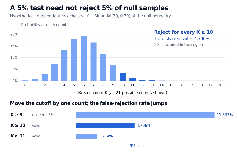
Exact binomial probabilities with counts 10 through 20 in the rejection region; its size is 4.796%, compared with 11.333% at cutoff 9 and 1.714% at cutoff 11.
Original hypothetical independent-check model, evaluated at the worst-case null boundary p=0.30. Integer counts make achievable false-rejection probabilities jump; the cutoff 10 is included.
This is a level-5% test with actual size about 4.796%. A level is a bound; it need not be attained exactly. Reducing the cutoff to 9 would overshoot the bound. Raising it to 11 is valid but rejects less often, including when the breach rate truly exceeds the benchmark, reducing power. Among these upper-tail cutoff rules, 10 keeps the largest rejection region allowed by the 5% constraint. This comparison concerns nonrandomized rules: a separate random decision at a boundary count could fill the remaining probability budget, but is not part of this test.
The inequality is substantive. Ten breaches reject under K≥10. Writing K>10 would instead mean K≥11 and change the size to 1.714%. Continuous reference distributions assign probability zero to a single cutoff; a discrete count can assign it substantial probability.
Fixed region, observed p-value
Once the test is fixed, its rejection region stays {10,…,20} whether the desk observes 9, 10 or 11 breaches. The p-value changes with the observed count kobs. For this upper-tail composite-null test it is
0≤p≤0.30supPp(K≥kobs)=P0.30(K≥kobs).
Nine breaches give approximately 0.11333 and do not reject; ten give 0.04796 and reject; eleven give 0.01714 and reject. With the stated convention, comparing this p-value with 0.05 using ≤ reproduces membership in the fixed region. The p-value is an observed tail probability, while the test's size describes the probability of entering its fixed region under the worst-case null. They coincide here when the observed count is exactly the included cutoff, not for every possible result.
The shape must follow the question
An upper-tail region fits “too many breaches.” A lower-tail test looks for unexpectedly small values. A two-sided test allows departures in either direction; its region can have two separated pieces. “Rejection region” does not mean one contiguous interval, and “two-sided” does not universally mean equal probability in each tail, especially for asymmetric discrete laws.
For a continuous mean-test comparison, Confidence Intervals and Hypothesis Testing derives a two-sided normal-family rejection rule and connects it to an interval. The public page is a preview; the full lesson requires membership.
The Type I error guarantee comes from the sampling model and the complete testing protocol. Dependent risk checks need not have this binomial law. Repeatedly testing until a breach occurs, or choosing the direction after seeing the count, changes the procedure and requires its own calibration. Finally, falling outside the region means failure to reject the null; it does not establish that the breach rate is acceptable.
Sources
John A. Rice, Mathematical Statistics and Data Analysis, 3rd edition (Duxbury, 2007), §§9.2–9.2.1: rejection regions, null distributions and p-values.
George Casella and Roger L. Berger, Statistical Inference, 2nd edition (Duxbury, 2002), §8.3.1, Definitions 8.3.5–8.3.6: actual size and level bounds.