A directional hypothesis test for a positive mean return: choose the tail in advance, calculate its p-value, and control error across the composite null.
One-sided test
A one-sided test is a hypothesis test whose alternative specifies a direction, such as a mean return above a benchmark. Its rejection region targets evidence in that direction. An extreme result in the opposite direction does not support the chosen alternative.
For a strategy researcher, “is expected excess return positive?” is a different question from “does expected excess return differ from zero?” Choosing the first question before examining the data allows the entire false-rejection allowance to be spent on positive evidence. Choosing it because the backtest happened to look positive undermines that allowance.
Commit to the direction
Let μ denote a fixed strategy's mean daily excess return, after specified costs and relative to a specified cash benchmark. A positive-edge question uses
H0:μ≤0,H1:μ>0.
The null includes zero and every negative mean. This is a composite null: it contains several possible parameter values. For a cost-reduction question the desired direction might instead be downward, using H0:μ≥μ0 against H1:μ<μ0. The economic question determines the direction; the observed sign does not.
A positive average, tested in its declared direction
Consider an original hypothetical experiment with 64 daily excess returns. Stipulate independent, identically distributed normal observations, a known population standard deviation of 1 percentage point (pp), and an observed sample mean of 0.25 pp per day. These are teaching assumptions, not measured properties of a trading strategy. Fix the strategy, sample window, hypotheses and 5% significance level before inspecting the results.
The standard error of the mean is 1/64=0.125 pp. Standardizing against the null boundary gives
zobs=0.1250.25−0=2.
At μ=0, the random statistic Z=Xˉ/(σ/n) has the standard normal distribution. Write Φ for its cumulative distribution function. The right-tailed p-value is
p=1−Φ(2)≈0.02275013.
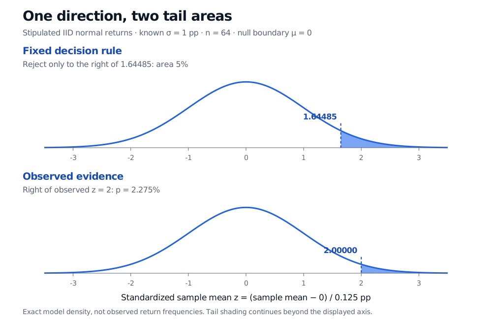
The predeclared 5% rule rejects when zobs>Φ−1(0.95)≈1.64485, equivalently when p<0.05. Here it rejects: the sample provides evidence for a positive mean under the stipulated model. The p-value is not the probability that the strategy has no edge, and rejection does not establish persistence or economic value.
Why is zero the reference when the null includes negative means? Holding the standard deviation and sample size fixed, shifting the true mean downward makes a large positive sample mean less likely. The rejection probability is largest at the boundary μ=0, where it is exactly 5%; for every μ<0, it is smaller. Thus the rule controls false rejection throughout this composite null. This boundary argument relies on this model and rejection rule; it is not a universal shortcut for composite hypotheses.
At the zero-mean null boundary, the fixed right-tailed rejection region starts at z 1.64485 and has probability 5%. The observed z 2 has a smaller right-tail p-value of 2.275%.
Original exact normal-model calculation. The first panel shows the fixed rejection region; the second shows the observed p-value tail. Both use the same boundary-null density.
A matching 95% one-sided confidence bound supplies an effect-size statement:
L=xˉ−Φ−1(0.95)nσ=0.25−1.6448536(0.125)≈0.04439 pp.
The confidence set is [L,∞). Its lower endpoint is positive, agreeing with rejection of μ≤0. Over repeated samples under this model, this bound covers the fixed true mean 95% of the time. That is a property of the procedure, not a 95% probability assigned to the realized set. We use strict rejection and a closed bound: at an exact zero lower endpoint, the null is not rejected.
For the sampling laws and the change to Student's t when volatility is estimated, see Confidence Intervals and Hypothesis Testing (public preview; full lesson requires membership). “Known volatility” is a substantive assumption here; replacing it with a sample estimate changes the reference distribution.
The other tail is not a second chance
If the same design instead produced zobs=−2, its right-tailed p-value would be 1−Φ(−2)≈0.97724987. Even a very large negative result does not support μ>0. It may matter greatly for risk decisions, but that is separate from rejecting this null in favour of a positive edge. Failure to reject also does not prove the null.
A different, predeclared two-sided test of μ=0 against μ=0 would give 2[1−Φ(2)]≈0.04550026 for the original positive result. This doubled value answers a different question; it is not a penalty one may remove after seeing the sign. In this symmetric normal example, choosing whichever one-sided 5% test favours the observed sign rejects in either 5% tail. At zero mean, its false-rejection probability is therefore 10%.
Direction is only one part of the research design. Searching many strategies, changing the stopping date, serially dependent returns or a poorly estimated sampling variance can invalidate the stated error control. A one-sided rule does not repair those problems.
John A. Rice, Mathematical Statistics and Data Analysis, 3rd ed., Duxbury, 2007, §§9.2.1–9.2.3 and 9.3. Significance levels, composite hypotheses, one-sided normal-mean tests and interval/test duality.