Use Student’s t-test to compare a mean with a benchmark, interpret a return example, and choose between one-sample, paired, pooled and Welch designs.
Student's t-test
Student's t-test is a hypothesis test for a population mean, or a difference of means, that divides an estimated effect by its estimated standard error and compares the result with a Student t distribution. The name covers several related tests; the assumptions and degrees of freedom depend on the design.
For a quant researcher, it answers a specific question: is the observed average return unusually far from a predeclared benchmark, relative to the uncertainty in that average? It does not establish that a strategy will remain profitable, and the familiar t reference is exact only under particular sampling assumptions.
One mean, an estimated denominator
Suppose X1,…,Xn are independent observations from one normal population with mean μ and unknown positive variance σ2. For the null hypothesisH0:μ=μ0, use
T=S/nXˉ−μ0,S2=n−11i=1∑n(Xi−Xˉ)2.
Here Xˉ is the sample mean, S is the sample standard deviation, and S/n estimates the standard error of the mean. Under the null and these normal-sampling assumptions,
T∼tn−1.
The numerator measures distance from the benchmark. The denominator puts that distance on an uncertainty scale. Estimating the population standard deviation from the same sample creates the extra tail uncertainty accounted for by the t law. Rice's normal-sample derivation establishes the required independence of the mean and sample variance; substituting a sample standard deviation into an arbitrary statistic does not automatically produce a t distribution.
At significance level α, reject when ∣tobs∣>tn−1,1−α/2, where the second subscript denotes a lower-CDF quantile. This uses the strict rejection convention; an exact boundary is retained in the matching closed confidence interval. NIST's one-population mean reference sets out the statistic and the different tail choices.
A positive weekly average, still compatible with zero
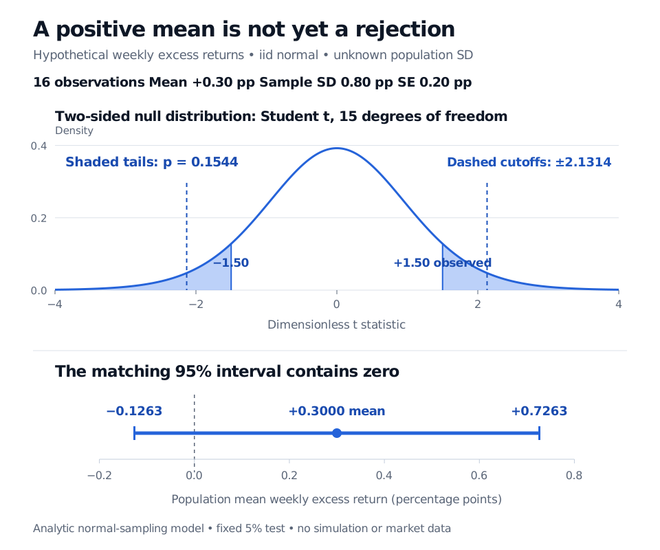
Consider a hypothetical, predeclared study of 16 weekly excess returns. Assume iid normal sampling for this teaching example; this is not a claim about observed financial returns. The recorded summaries are a mean of +0.30 percentage points and a sample standard deviation of 0.80 percentage points. All return quantities below use percentage points per week; the statistic itself has no units.
Test H0:μ=0 against H1:μ=0 at the 5% level:
SE=160.80=0.20,tobs=0.200.30−0=1.50,ν=15.
The two-sided p-value is 0.1544. The 5% two-sided cutoffs are approximately −2.1314 and +2.1314. Since 1.50 is between them, the test does not reject zero. A positive observed mean is not sufficient evidence of a positive population mean.
0.30±2.1314495(0.20)≈[−0.1263,0.7263]percentage points per week.
Zero lies inside it, consistent with the test decision. The interval also shows why “no significant difference” is not “no meaningful effect”: the sample is compatible with a range of negative and positive means. Its confidence level describes coverage of the procedure over repeated samples under the model, not a posterior probability assigned to this realised interval. NIST's mean-interval reference connects the interval with the matching two-sided test.
Analytic t15 null density: the tails beyond minus and plus 1.50 total p 0.1544; the 5% rejection cutoffs are minus and plus 2.1314. The corresponding 95% interval for mean weekly excess return is minus 0.1263 to plus 0.7263 percentage points, including zero.
Original analytic illustration under the stipulated iid normal model. Shading represents outcomes at least as extreme as the observed statistic; dashed lines mark the fixed 5% rejection cutoffs. The lower panel reports the same evidence in return units. The density continues beyond the displayed window.
The p-value is not a 15.44% probability that the null is true. Nor does it measure implementation costs, future drawdown or the probability of making money. To work through the normal-sample derivation and the distinction between significance and trading value, see Confidence Intervals and Hypothesis Testing. Its preview is public; the full lesson requires membership.
Which t-test matches the observations?
Design
What is tested and what must be justified
One sample
A population mean versus a benchmark. The exact reference above needs iid normal observations and uses n−1 degrees of freedom.
A mean of within-pair differences: for example, strategy A minus B in each matched week. It is a one-sample test on those differences. Exact inference needs iid normal differences; the two returns within a pair may be dependent.
Pooled two-sample t-test
A difference between two independent population means, with a common unknown variance. Independent normal samples and the common-variance assumption give an exact reference with n1+n2−2 degrees of freedom.
A difference between two independent means without assuming equal variances. It uses separate variance estimates and Welch–Satterthwaite degrees of freedom; its t reference is generally an approximation, even for normal samples.
Two strategies measured over the same market weeks are not automatically independent samples. Pairing preserves their common-week relationship rather than discarding it. Conversely, calling unrelated observations “paired” cannot create a matched design. NIST's two-sample reference distinguishes pairing and variance assumptions.
What the denominator cannot repair
With nonnormal iid observations and finite positive variance, Studentised mean inference can become approximately valid as the sample grows. There is no universal sample-size cutoff that makes severe skewness or rare extreme observations harmless. The exact small-sample result above does not apply to arbitrary return distributions.
Serial dependence is a separate issue: the standard error S/n ignores cross-observation covariance. Overlapping returns, changing volatility and nonstationary strategy behaviour require a sampling argument and an uncertainty estimate suited to that setting. Changing a predeclared two-sided test to a favourable one-sided alternative after seeing the sign, or reporting only the best result from many tested strategies, also changes the intended error control. The reference distribution alone cannot correct a research-selection process.
A useful report therefore states the estimated effect and its units, the sampling design, the standard-error method, the chosen alternative, the reference distribution and the uncertainty interval. A solitary t statistic hides too much of the claim.
Sources
John A. Rice, Mathematical Statistics and Data Analysis, 3rd ed. (2007), §6.3, Theorem B and Corollary B; §11.2.1, independent-sample t procedures and the unequal-variance approximation; §11.3.1, paired normal-sample inference.