Compare two independent means without assuming equal population variances. Work through the Welch standard error, fractional degrees of freedom and approximate confidence interval.
Welch's t-test
Welch's t-test compares the means of two independent populations without assuming that their population variances are equal. It divides the observed mean difference, after subtracting a hypothesised difference, by its estimated standard error and uses an approximate Student t reference distribution.
For a quant researcher, a higher average return in one group is only the start of the comparison. The size and variability of both samples determine how precisely that mean gap is estimated. Welch's method lets a smaller or noisier group contribute its own uncertainty instead of pooling the two variances under a common-variance assumption.
The denominator does the work
Let group A contain nA observations and group B contain nB. Write their sample means as xˉA,xˉB, and their sample standard deviations as sA,sB. Each sample variance uses its own denominator ng−1.
The two variance contributions add because the groups are independent. The standard error has the same units as the observations; tW is dimensionless.
Keep this value fractional when evaluating the t distribution numerically. It measures the uncertainty in the estimated variance of the contrast, rather than simply counting all observations minus two. If one variance contribution dominates, its group's residual degrees of freedom become especially influential.
For a predeclared two-sided alternative, the approximate p-value is
where tν,q is the lower-CDF q quantile. The degrees of freedom come from the data, and the reference is approximate even with independent normal observations. Welch inference does not inherit the exact finite-sample t guarantee of the equal-variance pooled normal model. NIST gives the two-sample standard error and reference construction.
A small comparison in basis points
Consider two hypothetical, independently sampled groups of same-horizon strategy returns under a fixed design:
Group A: 1,2,3,4,5 basis points.
Group B: −1,0,1,2 basis points.
For this teaching example, assume observations are independent within each group and between groups, with normal sampling in each population and unknown positive variances. These assumptions are stipulated, not inferred from nine observations. The rows are separate groups, not matched dates.
Quantity
Group A
Group B
Sample size
5
4
Mean, bp
3
0.5
Sample variance, bp squared
5/2
5/3
Contribution to variance of the mean gap, bp squared
1/2
5/12
Testing Δ0=0 against a two-sided alternative gives
At a prespecified 5% significance level, this rejects a zero mean difference using the approximate Welch reference. With tν,0.975≈2.365945, the corresponding 95% interval is
2.5±2.365945(0.957427)≈[0.234780,4.765220] bp.
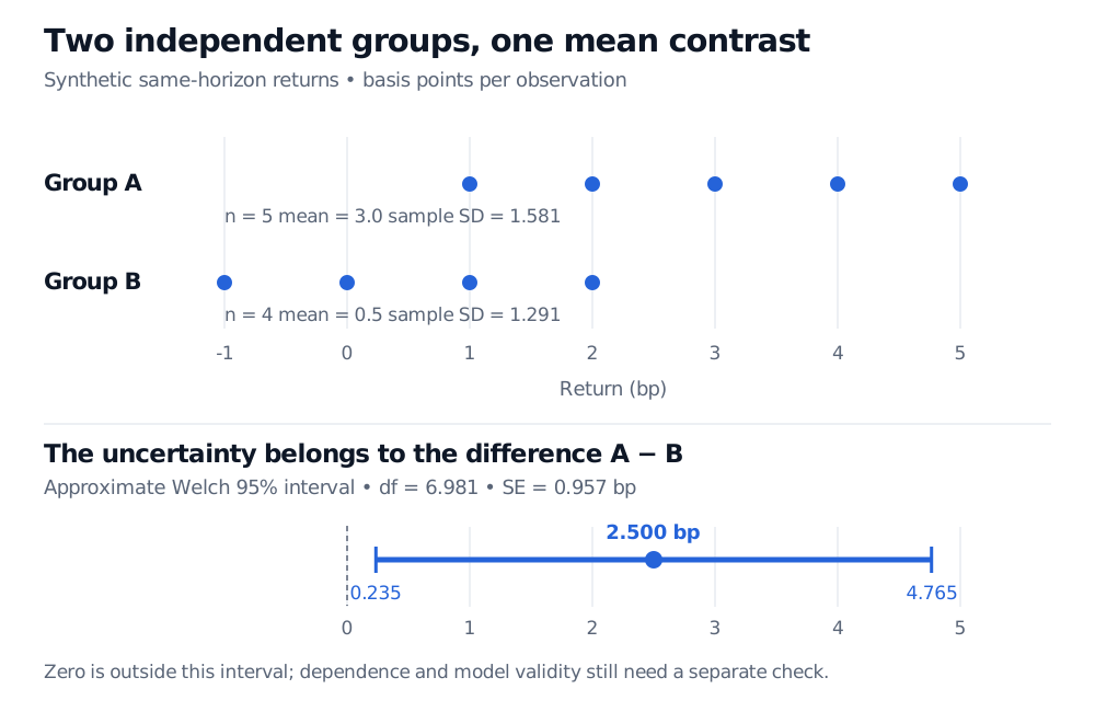
Independent group returns in basis points: A has mean 3 and B has mean 0.5. The difference is 2.5 bp with SE 0.957 bp, df 6.981 and approximate 95% Welch interval 0.235 to 4.765 bp.
Original synthetic example. Separate rows carry no pairing. The lower panel estimates the population mean difference using the stated sampling model and the approximate Welch reference.
The interval excludes zero, but spans a wide range of possible effect sizes. Statistical significance does not establish that the difference survives transaction costs, a new market regime or selection among many tested strategies. Nor is 0.034939 the probability that the null is true.
For the underlying interpretation, Confidence Intervals and Hypothesis Testing develops the one-sample t argument, connects tests with intervals and explains the significance trap. It has a public preview; the full lesson requires membership.
Choose the design before the formula
Unequal variances are allowed; dependence is a different problem. When two strategies run on the same dates, common market shocks can make their returns dependent. A paired t-test instead analyses matched differences when that design is appropriate. Serial dependence within either group also changes the sampling uncertainty. Welch's denominator supplies no correction for either kind of dependence.
A variance pretest is not an entry requirement. Welch can be selected in advance without first rejecting equality of variances. Failure to reject equal variances does not establish them, and choosing between pooled and Welch tests after an unadjusted preliminary test adds a selection step. R's two-sample t-test uses Welch by default. In SciPy's independent-samples test, Welch requires setting equal_var=False; its default assumes equal variances.
Normality matters most in short samples. For large independent samples with finite variances and suitable central-limit conditions, mean inference can be approximately justified beyond normal populations. Strong skew, extreme outliers and very small groups can make the approximation unreliable. More observations, a defensible sampling design and a method suited to the data matter more than a precise-looking fractional degree of freedom.
Sources
John A. Rice, Mathematical Statistics and Data Analysis, 3rd ed. (2007), §11.2.1, pp. 421–428: independent normal-sample contrasts and the unequal-variance t approximation. The numerical calculations here retain fractional degrees of freedom rather than using integer table lookup.