A paired t-test tests a claim about the population mean of the differences between matched observations. It is a one-sample Student’s t-test applied to those differences. For a quant comparing two execution algorithms on the same market scenarios, the relevant observation is each scenario’s cost saving, rather than two unrelated lists of costs.
Pairing preserves a common context: the same trading day, instrument, customer or experimental unit. Dependence within a pair is allowed. The usual exact test requires the differences to be independent and identically normally distributed across pairs. Normality is a condition on the differences, not a requirement that the two cost series each pass separate normality tests.
Turn two measurements into one observation
Choose the subtraction order before interpreting the result. Write
If and are execution costs, a positive difference means B is cheaper. The null hypothesis can specify any benchmark , with zero representing no mean saving:
For complete pairs, compute the sample mean and sample standard deviation of the differences:
The standard error is , giving
Under , iid normal differences with positive population variance give a Student’s t-distribution with degrees of freedom. There are observations for inference, because each pair supplies one difference. With fewer than two pairs, or zero observed difference variance, this ordinary statistic is undefined.
For a two-sided test, the p-value is the probability, under the null model, of a t statistic at least as large in absolute value as the observed one. A one-sided alternative is also possible, but its direction must be chosen before inspecting the results.
Six matched execution scenarios
Consider these hypothetical costs, measured in basis points of traded notional. The pairing is fixed by scenario identity; the numbers illustrate the calculation rather than establish a real trading advantage.
| Scenario | A cost (bp) | B cost (bp) | Saving A − B (bp) |
|---|---|---|---|
| 1 | 2 | 2 | 0 |
| 2 | 3 | 2 | 1 |
| 3 | 2 | 1 | 1 |
| 4 | 5 | 3 | 2 |
| 5 | 4 | 2 | 2 |
| 6 | 6 | 3 | 3 |
The six differences have mean bp and sample variance . Therefore,
Using five degrees of freedom, the two-sided p-value is approximately . A prespecified test rejecting when rejects the zero-mean null under the stated model. The matching 95% confidence interval for the mean saving is
where denotes the 97.5th percentile. This interval excludes zero and reports the size and uncertainty of the estimated saving. It is an interval for the population mean saving, not a guarantee that B saves money in each new scenario. Six observations provide little information with which to assess the distributional assumption; the attractive p-value does not validate that assumption.
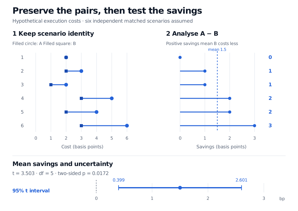
Original hypothetical matched-cost example. The left panel preserves scenario identity; the right panel isolates savings. The lower interval uses six iid normal differences as the inference model.
Why matching can improve precision
Within-pair covariance enters the variance of a difference:
When both algorithms face unusually difficult conditions in the same scenario, their costs may rise together. Positive covariance can cancel part of that shared noise when costs are subtracted. Negative covariance instead increases difference variance. Positive correlation is a potential precision benefit, not a validity requirement for the paired test.
For the paired-interval derivation and the variance comparison with an independent-sample design, see the paired-sample section of Two-Sample Tests and Intervals (public preview; full lesson requires membership).
Preserve the design, not just the row count
- Keep the real match. Sorting A and B separately before subtracting destroys the scenario match and can manufacture an artificially small difference variance. Reordering matched rows together is harmless. Any complete one-to-one re-pairing preserves ; it can still change , the statistic and the p-value. A fixed, data-independent pairing of genuinely independent iid normal samples can produce a valid one-sample t test on differences, but supplies no covariance benefit.
- Check dependence across pairs. Pairing two strategies by trading day preserves their same-day relationship; it does not remove autocorrelation across days. Overlapping returns or repeated orders within the same market event can invalidate . The uncertainty calculation then needs a method suited to that dependence.
- Check the difference series. Outliers and heavy tails matter, especially with few pairs. Under suitable finite-variance conditions, large-sample inference can be approximately valid without normality; there is no universal pair count that repairs arbitrary skewness, dependence or tail behaviour.
- Separate mean evidence from a deployment decision. Statistical significance does not establish causality, stability after strategy selection, or savings large enough to cover switching costs. A before/after pairing can still confound a system change with a market-regime change.
Sources
- John A. Rice, Mathematical Statistics and Data Analysis, 3rd ed. (Duxbury, 2007), §§11.3–11.3.1, pp. 444–446: paired-design covariance, reduction to differences and normal-theory inference.
- NIST/SEMATECH e-Handbook, §7.3.1.1: Analysis of paired observations: matched observations, difference summaries and t reference tests.
- SciPy documentation:
ttest_rel: related-sample test, sign convention, degrees of freedom and confidence interval.