Statistical significance is a thresholded test result under stated assumptions. A synthetic return example separates a tiny p-value from effect size and profit after costs.
Statistical significance
Statistical significance means that a result crosses the rejection threshold of a specified hypothesis test. With a prechosen significance level α, the usual p-value rule calls a result significant when p<α. This article uses strict rejection; an equality convention should be stated when it can matter.
The label is conditional on the null hypothesis, test direction, sampling model and analysis procedure. It does not measure how profitable, large, causal or repeatable an effect is. In quantitative research, confusing those questions can turn a convincing statistical result into a poor trading decision.
The threshold is a procedure, not a probability of truth
The p-value is a tail probability calculated under the specified null model: how often would a statistic at least as extreme as the observed one occur? The significance level is chosen before examining the result. A valid level-α procedure controls the probability of rejecting a true null at no more than α, over repeated applications under its assumptions.
Consequently, a 5% significance level does not mean that a particular rejected null has a 5% probability of being true. Nor does it mean that only 5% of reported significant findings are false. Those are different conditional questions; the latter also depends on which hypotheses were tested and how findings were selected. The ASA's six principles explicitly distinguish p-values from posterior probabilities and effect importance.
The cutoff also creates a discontinuous label from a continuous measure. Two otherwise comparable results barely on opposite sides of the threshold do not suddenly have radically different evidential strength. Report the estimate, its uncertainty and the p-value alongside the decision.
A strong gross result that does not pay its costs
Consider a synthetic study of one fixed strategy and one predeclared analysis. Returns have a common observation horizon; all quantities below use that same horizon. Stipulate 10,000 independent, identically distributed normal returns with unknown mean μ and known population standard deviation of 1 percentage point (pp). The observed mean gross return is 0.05 pp. These are teaching assumptions, not a claim about actual market data.
Test H0:μ=0 against H1:μ=0 at α=0.05. The standard error and observed statistic are
SE=10,0001 pp=0.01 pp,z=0.01 pp0.05 pp−0=5.
Under this null, the statistic has a standard normal distribution exactly. Writing Φ for its cumulative distribution function,
p=2[1−Φ(5)]≈5.7330×10⁻⁷<0.05.
The gross mean is statistically significant. This tiny p-value concerns the zero-gross-mean null under the stipulated model; it is not the probability that the strategy will lose money.
Now stipulate a fixed trading cost of 0.08 pp per observation horizon, charged on the same return basis. The point estimate after costs is
0.05 pp−0.08 pp=−0.03 pp.
The same data can therefore produce strong evidence against zero gross mean and a negative estimated net return. Testing the wrong economic benchmark precisely does not make it the right benchmark.
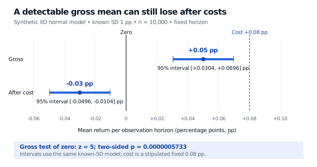
Synthetic known-SD normal example: gross mean +0.05 pp has a 95% interval +0.0304 to +0.0696 pp, above zero but below a fixed +0.08 pp cost. After subtracting cost, the mean is −0.03 pp and the interval is −0.0496 to −0.0104 pp.
Original synthetic calculation. Both intervals use the same normal model and known SD; the net interval is the gross interval shifted by the stipulated fixed cost.
The matching 95% confidence interval for gross mean return is approximately [0.0304,0.0696] pp. It excludes zero, agreeing with the two-sided 5% test, but lies entirely below the cost benchmark. Subtracting the fixed cost gives [−0.0496,−0.0104] pp for net mean return. If costs were estimated or varied with trading conditions, their uncertainty and relationship with gross returns would also belong in the analysis.
For the underlying sampling laws and the test–interval connection, read Confidence Intervals and Hypothesis Testing (public preview; full lesson requires membership). When population SD is estimated rather than known, the exact normal-sample mean test uses Student's t distribution instead.
What survives outside the model?
A large sample can make a small effect statistically detectable because the standard error shrinks with the square root of sample size under this model. That improves precision; it does not increase the effect's economic magnitude. Conversely, failure to reject zero can reflect imprecision rather than absence of an effect. Study power against economically relevant alternatives before interpreting a non-significant result as reassuring.
Financial observations may overlap, be serially dependent or follow changing regimes. Counting dependent returns as independent can misstate uncertainty; a large observation count alone does not validate the standard error. Checking assumptions is part of the inference, not something the significance label certifies.
Selection matters too. Testing many strategy variants and reporting only the winner changes the research procedure. Multiple testing and repeated peeking can invalidate the intended error control unless the design accounts for them. A significant association also does not establish causation, and a new sample can behave differently. A useful research report names the tested benchmark, effect size, uncertainty, costs, search history and validation design rather than ending with an asterisk.
Sources
John A. Rice, Mathematical Statistics and Data Analysis, 3rd edition, §9.2.1, “Specification of the Significance Level and the Concept of a p-value.”