Fit a fund-return line from five synthetic weeks, interpret slope and intercept units, and distinguish OLS geometry from assumptions about conditional means, uncertainty and forecasts.
Simple linear regression
Simple linear regression models a quantitative response using one predictor and a straight-line mean relationship. In its usual form,
Y=β0+β1X+ε,E[ε∣X]=0,
so the conditional expectation is E[Y∣X=x]=β0+β1x. The intercept β0 gives the mean response at x=0; the slope β1 gives the change in that mean per unit increase in x. “Simple” means one predictor, even though the model has two coefficients.
On a risk desk, X could be the market's weekly excess return and Y a fund's excess return over the same week. The slope describes market exposure; the intercept describes the mean component at zero market excess return. Neither coefficient, by itself, establishes a trading opportunity.
A population relationship and a line fitted to data
The population coefficients are unknown. From observed pairs (xi,yi), a fitted line uses estimates:
y^i=β^0+β^1xi,ei=yi−y^i.
The residualei is an observable vertical difference from the fitted line. The model error εi=Yi−β0−β1Xi is a deviation from the unknown population line. These are different objects: changing the sample changes the estimates and residuals, even when the population relationship stays fixed.
One can always fit a straight line to nonconstant observed x values. Doing so does not establish that the population conditional mean is straight. If that mean is curved, a fitted line can still summarise linear association, but its slope is not a constant change in the true conditional mean across all x. A general linear regression is linear in its coefficients; the straight-line, one-predictor case here is the simplest instance.
Five weeks, with the units left visible
A researcher wants to describe a fund's exposure after five completed weeks. The following excess returns are synthetic, aligned to the same weeks and measured relative to the same weekly risk-free return. A table entry of −2 means a return of −2%; a difference of one between entries is one percentage point (pp).
Week
Market x (%)
Fund y (%)
Fitted y^ (%)
Residual e (pp)
1
−2
−1
−1.4
+0.4
2
−1
0
−0.2
+0.2
3
0
0
1.0
−1.0
4
1
2
2.2
−0.2
5
2
4
3.4
+0.6
Ordinary least squares, or OLS, chooses the intercept and slope to minimise the sum of squared vertical residuals:
a,bmini=1∑n(yi−a−bxi)2.
It holds each xi fixed while measuring the miss in y. It does not minimise the shortest geometric distance from each scatterplot point to the drawn line; treating both coordinates as noisy measurements requires a different modelling decision.
For an unweighted fit with an intercept, define
SxxSxy=i∑(xi−xˉ)2,=i∑(xi−xˉ)(yi−yˉ).
If Sxx>0, the unique OLS coefficients are
β^1=SxxSxy,β^0=yˉ−β^1xˉ.
Here xˉ=0, yˉ=1, Sxx=10 and Sxy=12. Hence
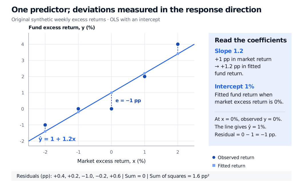
β^1=1.2,β^0=1,y^=1+1.2x.
The slope means a one-percentage-point larger market return is associated with a 1.2-percentage-point larger fitted fund return. Because both returns use the same units, the ratio is dimensionless. It is a fitted market beta for this sample, rather than proof of a stable population exposure or of the CAPM's pricing restrictions.
The intercept is a fitted weekly excess return of 1% when the market's excess return is 0%. It is not a guaranteed 1% weekly payoff. In an excess-return factor regression it is often called estimated alpha, but five observations cannot establish repeatable skill, compensation unexplained by other risk factors, or a positive net return after costs. If zero lies far outside the observed predictor range, even the intercept's descriptive interpretation involves extrapolation.
Five synthetic weekly market and fund excess-return pairs. The OLS line is y-hat = 1 + 1.2x in percent units. At market return zero, the fitted fund return is 1 percent, the observed fund return is zero, and the vertical residual is minus 1 percentage point. The five squared residuals sum to 1.6 percentage points squared.
Original synthetic weekly sample. Filled circles are observed returns, filled squares are fitted returns, and dashed vertical segments are residuals. Coefficients describe this sample.
Changing both return series from percent to decimals changes the equation to y^=0.01+1.2x: the intercept rescales, while the slope stays 1.2. Changing only the predictor's units changes the numerical slope as well; if x alone is a decimal return and y stays in percent units, the equation is y^=1+120x. Report the units alongside the coefficients.
For a slower introduction to the same mechanics, Basic Statistics and Regression develops sample summaries, fitted lines and vertical residuals. Its full lesson is available with a free signed-in account; the public page provides a preview.
Why the residuals balance, even for a bad model
Differentiating the OLS objective with respect to the intercept and slope gives the normal equations:
i∑ei=0,i∑xiei=0.
The first makes the fitted line pass through (xˉ,yˉ). The second makes the residual vector orthogonal to the observed predictor vector. Both are consequences of fitting an intercept and slope by OLS on these observations. They require no normality assumption and do not certify a correct model. A curved relationship can leave conspicuous curvature in the residuals while still satisfying both identities.
In vector form, every possible fitted response has the form a1+bx. OLS projects the observed vector y∈Rn onto the space spanned by 1 and x. The leftover vector e is perpendicular to that space. This perpendicularity is in observation space; the scatterplot's individual residual segments remain vertical.
For the five weeks, the residuals sum to zero, their products with x sum to zero, and
SSE=0.42+0.22+(−1)2+(−0.2)2+0.62=1.6.
SSE has units of pp squared. The centred total sum of squares is ∑i(yi−yˉ)2=16 pp squared, so the coefficient of determination is R2=1−1.6/16=0.90. That is a 90% reduction in squared error relative to predicting the sample fund mean of 1% on these same weeks. It is neither a success probability nor a forecast accuracy guarantee.
Two boundary cases clarify what the formulas need. If every predictor value is identical, then Sxx=0: the sample cannot separately identify a slope and intercept, although the constant fitted response at that observed predictor is the response mean. If x varies but every y is identical, OLS gives slope zero and a perfect constant fit; centred R2 is undefined because its denominator is zero.
What must hold beyond the minimisation
There are several separate claims a researcher might want to make:
“These coefficients minimise sample squared error.” Nonconstant finite x and a free intercept suffice; stochastic assumptions are unnecessary.
“They estimate this population mean relationship without conditional bias.” For a fixed design, or conditional on the full observed design, use the correctly specified model and E[ε∣X]=0. Zero sample residuals do not establish this condition. Omitted drivers correlated with the predictor, measurement error and selection can undermine the intended interpretation.
“The usual standard errors and exact tests are valid.” The classical variance calculation additionally assumes equal conditional error variance and no cross-observation error covariance. Exact Gaussian regression tests require independent normal errors conditional on the design, with common variance. Marginal normality of returns is insufficient.
Finance data particularly warrant checks for changing residual spread (heteroskedasticity), time dependence (autocorrelation), curvature, and observations that dominate the slope. Look at residuals against the predictor, fitted values and time; inspect sensitivity to unusual observations. Appropriate robust uncertainty estimates can address certain variance or dependence problems, but cannot turn an incorrect conditional mean or an endogenous predictor into a causal model. A larger sample alone does not repair those problems.
The Linear Regression lesson derives the normal equations and projection picture, then develops inference under explicit assumptions. It has a public preview; full access requires membership.
Exposure today is not a forecast issued yesterday
In this example, market and fund returns cover the same week. Knowing the market's realised return helps describe the fund's realised exposure; that market return was unavailable at the start of the week. Substituting it into a purported start-of-week forecast introduces look-ahead bias.
A forecasting regression must use predictors available when the forecast is issued and must be evaluated on later observations with an explicit benchmark. Choosing the sample, specification or trading rule after seeing those later outcomes can still produce overfitting. The Forecast Evaluation lesson explains forecast origins, evaluation loss and benchmark comparisons; a public preview is available and the full lesson requires membership.
Nor does a fitted slope identify the effect of intervening on X. Common drivers, reverse causation and selection can generate association. Simple regression is useful when one predictor is a deliberate approximation to the research question; moving to multiple linear regression can represent additional drivers, but causal identification, observation timing and regime stability still require their own arguments.
Sources
Gareth James, Daniela Witten, Trevor Hastie and Robert Tibshirani, An Introduction to Statistical Learning: with Applications in R, 2nd edition (2021), §§3.1–3.1.2, pp. 61–68 — one-predictor regression, least-squares estimation, and the distinction between population and fitted lines. Authors' book site.