Read regression slopes and intercepts through a fund-return example, track their units under rescaling, and distinguish association, partial relationships, causal effects and forecasts.
Regression coefficient
A regression coefficient is a number multiplying a predictor in a regression model; the constant term is the intercept coefficient. In a straight-line model, the slope tells you how much the fitted response changes for a one-unit increase in the predictor. Its meaning depends on the predictor, the response, their units and the other variables in the model.
For a risk analyst, a fund's coefficient on market returns can describe its historical market exposure. A coefficient on yesterday's information in a forecasting model answers a different question. Neither coefficient, by itself, establishes a causal effect or a profitable trade.
Here xi is the predictor and yi the response for observation i. The population coefficients are β0 and β1; hats mark estimates obtained from the sample. The model error εi is distinct from the fitted residual, ei=yi−y^i.
The slope describes the fitted line, not an exact change in every observed outcome. If the population conditional mean is genuinely linear and the error has conditional mean zero, β1 also describes the change in that conditional mean. Least squares can still fit a line when those assumptions fail; the calculation alone does not establish them.
Ordinary least squares chooses the coefficients to minimise the sum of squared residuals. With an intercept and a nonconstant predictor,
The ratio uses sample covariance and sample variance calculated on the same matched rows with the same divisor. If every xi is identical, an intercept and slope cannot be separately identified.
A risk desk's five-week fit
Suppose a desk records these synthetic weekly simple returns for a market and a fund. The observations cover the same weeks; both are total returns in the same currency, without risk-free subtraction. Entering 2 means a return of 2%.
Week
Market x (%)
Fund y (%)
Fitted fund (%)
Residual (percentage points)
1
−2
−1
−1.4
+0.4
2
−1
0
−0.2
+0.2
3
0
0
1.0
−1.0
4
1
2
2.2
−0.2
5
2
4
3.4
+0.6
The means are xˉ=0 and yˉ=1. The centred cross-product sum is 12 and the centred squared-market-return sum is 10, both in squared percentage-point units. Consequently,
β^1=12/10=1.2,β^0=1,y^=1+1.2x.
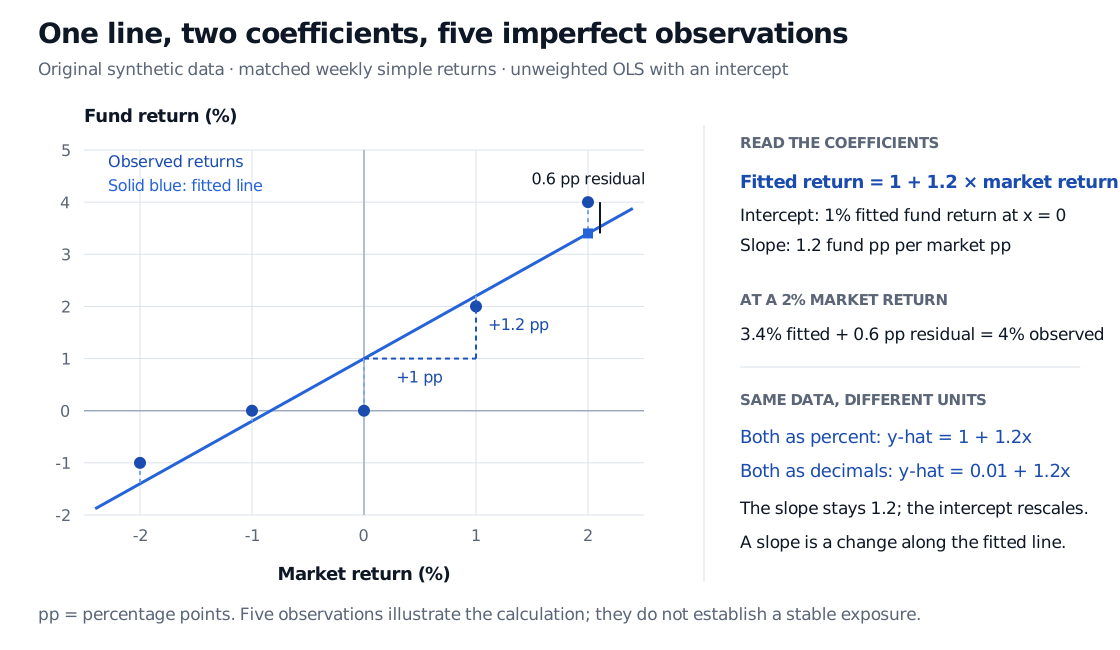
A one-percentage-point increase in market return corresponds to a 1.2-percentage-point increase along the fitted fund-return line. At a market return of 2%, the fitted fund return is 3.4%. The observed 4% return exceeds it by 0.6 percentage points. The slope 1.2 and the residual 0.6 measure different things.
Five synthetic weekly return pairs fitted by an intercept of 1% and slope of 1.2 fund percentage points per market percentage point. At market return 2%, fitted fund return is 3.4%, observed return is 4%, and the residual is +0.6 percentage points. Converting both series to decimals preserves slope 1.2.
Original synthetic matched-week example. The dashed triangle measures a change along the fitted line; vertical dashed gaps show residuals. The intercept and residuals change units when both return series are rescaled, while the slope stays the same.
The intercept is the fitted fund return when the market return is zero. It is not necessarily the realised return in a zero-market week: week 3 has a residual of −1 percentage point. In this raw-return specification, calling the intercept “alpha” would require additional choices about the risk-free rate, benchmark factors and performance model. A weekly intercept also does not automatically become an annual performance measure by multiplication or compounding. Changing the return horizon changes the statistical problem.
A coefficient carries units
The slope's units are response units per predictor unit. Its numerical size is therefore not a universal measure of importance.
Input convention for the same observations
Intercept
Slope
Meaning of a one-unit predictor change
Both returns as percent numbers
1
1.2
1 market percentage point
Both returns as decimals
0.01
1.2
A market decimal return change of 1, or 100 percentage points
Market as decimal; fund as percent number
1
120
100 market percentage points
Market as percent number; fund as decimal
0.01
0.012
1 market percentage point
For example, the decimal version is y^=0.01+1.2x: inserting x=0.02 gives y^=0.034. That is the same fitted 3.4% return.
More generally, for pure nonzero rescalings x′=cx and y′=dy,
β^1′=cdβ^1,β^0′=dβ^0.
This differs from correlation, which removes positive scale changes. In simple OLS with an intercept and nonconstant response, β^1=rxysy/sx. A regression slope need not lie between −1 and 1. Standardising both variables produces a slope equal to their correlation in this specific simple-regression setting; it does not make a coefficient causal.
Adding predictors changes the question
In an additive multiple regression,
y^=β^0+β^1x1+⋯+β^pxp,
β^j describes a one-unit change in xjholding the other included predictors fixed. A market-only fund coefficient combines associations that can be separated differently after adding size, sector or interest-rate predictors. It is not generally the same as the market coefficient from that larger model.
“Holding fixed” describes a comparison inside the fitted model. It does not mean the analyst performed an intervention, held every omitted influence constant, or found enough observations for every hypothetical comparison. Correlated predictors can also make individual estimates unstable: multicollinearity affects how precisely their separate coefficients can be estimated.
The constant-change interpretation above assumes an additive level model. With an interaction or a squared predictor, the response change can depend on the other predictor values; a log-transformed response also needs its own interpretation. Read the model formula before reading the coefficient column.
Which benchmark matters?
A coefficient is an estimate, so its size should be considered alongside its standard error, sample period and modelling assumptions. Different decisions have different benchmarks:
Zero: testing a slope against zero asks whether the specified model supports a nonzero relationship. It does not test causality or trading profitability.
One: for a return-on-market slope, comparing with one asks about one-for-one exposure. A positive market beta need not be statistically distinguishable from one. A test against zero cannot answer that question.
A feasible forecast: predictive use requires later observations and predictors available when the forecast is issued. Compare forecast losses against a stated alternative, such as a mean estimated from training data, using identical dates and information. A contemporaneous market return is usually unknown before that week ends; fitting fund return against it is exposure analysis, not automatically a forecast.
Finally, R-squared describes fit, rather than the units or economic meaning of a coefficient. A large slope, a precise slope and a useful forecast are separate findings. Five illustrative weeks cannot establish any of their stability.
For fitting mechanics, Basic Statistics and Regression is free in full with a signed-in account. Linear Regression derives the normal equations and coefficient uncertainty; its full lesson requires membership. Both offer public previews.
Sources
James, G., Witten, D., Hastie, T. and Tibshirani, R. (2021). An Introduction to Statistical Learning: with Applications in R, 2nd edition, §§3.1–3.1.1, pp. 61–62, and §§3.2–3.2.1, pp. 71–73. Coefficient definitions, least-squares estimation and interpretation with several predictors.