Sample covariance: Definition & Examples

Sample covariance measures how two observed variables move together around their own sample means. For a risk analyst, it is the cross-asset input that turns separate asset variances into a portfolio variance. Positive covariance means above-mean observations tend to align with above-mean observations, and below with below; negative covariance means opposite-side deviations tend to dominate.

It is a statistic calculated from paired data, distinct from the population covariance it may be used to estimate. A sample supplies observations; a sampling model supplies the justification for inference beyond them.

Centre, multiply, then choose the divisor

For $n\ge2$ aligned pairs $(x_i,y_i)$ , let $\bar x$ and $\bar y$ be their sample means. The usual sample covariance is

s_{xy}=\frac{1}{n-1}\sum_{i=1}^{n}(x_i-\bar x)(y_i-\bar y).

Each row contributes a signed cross-product. Two deviations with the same sign contribute positively; opposite signs contribute negatively. Larger deviations receive more weight through their product. Covariance is symmetric:

s_{xy}=s_{yx}

. Setting

y_i=x_i

gives the sample variance.

The pairing is part of the definition. For returns, row $i$ must refer to matching start and end times, a common horizon and compatible return conventions. Independently sorting each series, shifting one series by a day or mixing closing times changes the question. A lagged relationship can be studied deliberately, but it is different from contemporaneous covariance.

Four paired returns, all positive

Suppose two assets have the following synthetic one-period simple total returns on four matching dates. Both returns use the same currency basis. The entries are percent returns; subtracting their means produces deviations in percentage points (pp).

Period	X return (%)	Y return (%)	X deviation (pp)	Y deviation (pp)	Product (pp²)
1	1	2	−1.5	−0.5	+0.75
2	2	1	−0.5	−1.5	+0.75
3	3	4	+0.5	+1.5	+0.75
4	4	3	+1.5	+0.5	+0.75

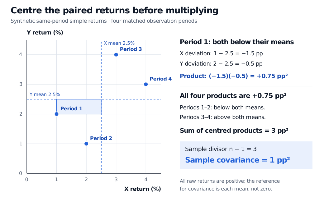
Both means are $2.5\%$ . Every pair lies on the same side of its two means, giving

\sum_{i=1}^{4}(x_i-\bar x)(y_i-\bar y)=3\text{ pp}^2, \qquad s_{xy}=\frac{3}{4-1}=1\text{ pp}^2.

Four synthetic return pairs (1%, 2%), (2%, 1%), (3%, 4%) and (4%, 3%), with both mean axes at 2.5%. Periods 1 and 2 are below both means, while periods 3 and 4 are above both. Each centred product is +0.75 pp², summing to 3 pp²; sample covariance is 1 pp². The highlighted period-1 rectangle has deviation side lengths 1.5 pp and 0.5 pp.

Original synthetic four-period example. The reference lines are sample means, not zero returns; the shaded rectangle illustrates one product of deviations.

Positive raw returns alone would not establish positive covariance. For example, two positive-return series could alternate between relatively high and low observations in opposite directions. The centring step distinguishes those cases.

Why $n-1$ — and when $n$ is appropriate

If the task is to describe the empirical distribution that puts equal probability $1/n$ on each observed pair, its covariance is

c_{xy}^{\mathrm{emp}}=\frac1n\sum_{i=1}^{n}(x_i-\bar x)(y_i-\bar y) =\frac{n-1}{n}s_{xy}.

That is $0.75\text{ pp}^2$ here. It is a legitimate descriptive quantity with a different divisor. Calling the four observations the entire finite collection of interest also makes this their population-of-observations covariance. Neither calculation needs independent observations simply to exist.

The

n-1

convention has an additional estimation property. If the random pairs

(X_i,Y_i)

are independent and identically distributed across rows, with finite second moments, then

\mathbb E[S_{XY}]=\text{Cov}(X,Y).

This unbiasedness does not require X and Y within a pair to be independent, or a normal distribution. It concerns the average estimate over repeated samples, not the accuracy of this one four-row estimate.

The reason can be seen from the centring identity

\sum_i(X_i-\bar X)(Y_i-\bar Y) =\sum_i(X_i-\mu_X)(Y_i-\mu_Y) -n(\bar X-\mu_X)(\bar Y-\mu_Y).

Under the stated assumptions, the first term has expectation $n\sigma_{XY}$ and the second $\sigma_{XY}$ , because $\text{Cov}(\bar X,\bar Y)=\sigma_{XY}/n$ . The expected centred sum is therefore $(n-1)\sigma_{XY}$ .

Selected histories, serial cross-dependence and changing distributions need separate analysis; dividing by $n-1$ does not automatically correct them. Even a well-defined historical estimate need not describe tomorrow's joint return distribution.

Units travel into portfolio risk

Covariance has product units: X units times Y units. Converting both series from percent entries to decimal returns divides each deviation by 100, so

1\text{ pp}^2=0.0001\text{ decimal-return}^2.

Doubling one series doubles covariance; adding a constant to either leaves it unchanged. Consequently, covariance magnitude is not a universal strength scale. Sample correlation divides by the two sample standard deviations, giving a dimensionless measure of linear association when both are nonzero. Here both sample variances are

5/3\text{ pp}^2

, so correlation is

1/(5/3)=0.6

The sample covariance matrix is

S=\begin{pmatrix}5/3&1\\1&5/3\end{pmatrix}\text{ pp}^2.

For equal period-start weights, held fixed within each period, portfolio simple returns are

(1.5,1.5,3.5,3.5)\%

. Assuming no external cash flows or unaccounted costs, their sample variance agrees with the portfolio variance calculation:

s_p^2=\mathbf w^\top S\mathbf w =\frac14\frac53+\frac14\frac53+2\left(\frac12\right)\left(\frac12\right)(1) =\frac43\text{ pp}^2, \qquad \mathbf w=\begin{pmatrix}1/2\\1/2\end{pmatrix}.

Using a common aligned sample across every column gives

S=Z^\top Z/(n-1)

, where

Z

contains column-centred observations. This construction is positive semidefinite: every fixed-weight sample portfolio has nonnegative variance. Pairwise deletion of missing data, using different rows for different matrix entries, can lose that guarantee. Common complete rows preserve the algebra, but deleting incomplete records can still change the population being represented.

To connect the calculation to a fitted hedge slope, Basic Statistics and Regression develops the ratio of sample covariance to predictor variance. Full access requires a free signed-in account; the public link provides a preview.

Sources

Mavrakakis, M. C. and Penzer, J. (2021). Probability and Statistical Inference: From Basic Principles to Advanced Models, first edition, §7.2.2, Definitions 7.2.7–7.2.10 and Claim 7.2.9: joint sample moments, covariance, scaling and variance of sums.
NIST/SEMATECH e-Handbook, §6.5.4.1: Mean Vector and Covariance Matrix: the sample covariance formula and matrix construction.
R Core, stats documentation: Correlation, Variance and Covariance: the $n-1$ convention for iid observations and the positive-semidefiniteness risk of pairwise missing-value handling.

Centre, multiply, then choose the divisor

Four paired returns, all positive

Why n−1n-1n−1 — and when nnn is appropriate

Units travel into portfolio risk

Sources

Related terms

Covariance

Missing data

Portfolio variance

Positive semidefinite matrix

Sample

Sample correlation

Sample standard deviation

Sample variance

Unbiased estimator

Why $n-1$ — and when $n$ is appropriate