Calculate sample correlation from matched return rows, see why centring matters and shared divisors cancel, and separate a historical coefficient from evidence about population dependence.
Sample correlation
Sample correlation is the Pearson coefficient calculated from a finite set of paired observations. It divides their sample covariance by the product of their sample standard deviations, giving a dimensionless measure of linear association between −1 and 1.
A portfolio analyst might calculate it from two assets' returns over the same holding periods. The result describes that history. Interpreting it as an estimate of an unknown population Pearson correlation requires a sampling model and a clearly defined target: which instruments, return convention, horizon and market conditions?
First make the rows mean the same thing
Suppose two hypothetical assets have the following four observed one-period simple returns. “P1” through “P4” identify the same start and end times for both assets. A value of 1 pp means a 1% return.
Matched holding period
Asset X (pp)
Asset Y (pp)
P1
1
2
P2
2
1
P3
3
4
P4
4
3
These rows are a synthetic historical sample, not four population scenarios with known probabilities. Pairing is part of the information: sorting each column independently would produce two identical columns and a spurious coefficient of 1. Identical marginal lists can have different correlations because correlation uses joint pairs.
Before calculating, check matching timestamps, time zones and return windows. A close-to-close return on one venue and a different closing window on another are not automatically comparable. State whether returns include distributions and whether currency conversion is part of the exposure. A stale quote can produce an apparent zero return without evidence that the underlying value was unchanged.
Centre, multiply, then standardise
For n≥2 paired observations with nonzero variation in each series, write xˉ and yˉ for their sample means. The coefficient is
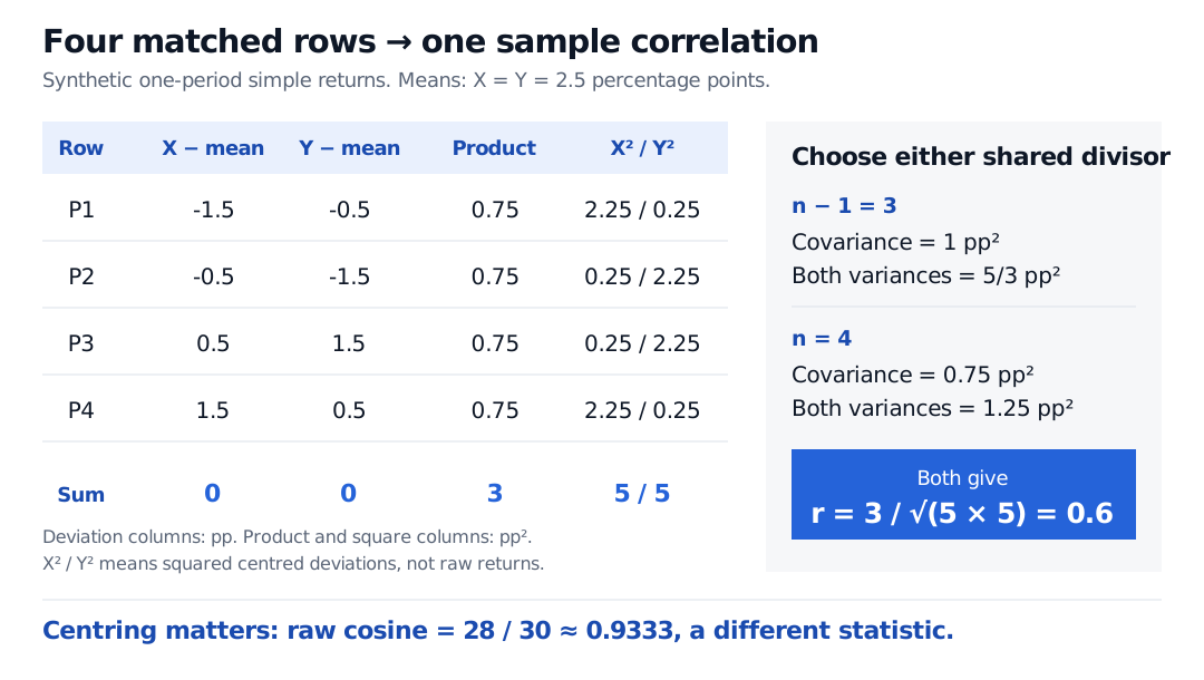
Each matched product is 0.75 pp², so the cross-sum is 3 pp². Each square-sum is 5 pp². Consequently,
r=553=0.6.
Centred-product ledger for four matched synthetic return rows: centred X values −1.5, −0.5, 0.5, 1.5 pp and centred Y values −0.5, −1.5, 1.5, 0.5 pp. All four cross-products are 0.75 pp squared, their sum is 3, and both squared-deviation sums are 5. Either common divisor gives correlation 0.6; the uncentred cosine is approximately 0.9333.
Original synthetic paired-return example. Every deviation uses the same four rows. The ledger shows why the divisor cancels and centring does not.
Using the usual n−1 convention gives sxy=1 pp² and sx2=sy2=5/3 pp². Using n consistently gives covariance 0.75 pp² and both variances 1.25 pp². The common divisor cancels in correlation; choosing n−1 does not make r an unbiased estimator. Mixing a covariance with one divisor and standard deviations with another gives the wrong ratio.
Centring cannot be skipped. The cosine of the raw observation vectors is 28/30≈0.9333, a different quantity. Pearson sample correlation measures alignment after subtracting each series' mean. Converting both return columns from pp to decimals changes covariance from 1 pp² to 0.0001 decimal-return squared and leaves r=0.6. Adding a constant also leaves r unchanged; multiplying just one series by a negative constant reverses its sign.
What the number can support
Here r>0 says above-mean X returns tend to accompany above-mean Y returns, and below-mean returns tend to accompany below-mean returns. It does not say that 60% of returns have matching signs, that X causes Y, or that future diversification will reproduce this history. The value is symmetric in X and Y and is not a regression slope.
The bound follows from Cauchy–Schwarz applied to the two centred vectors. If both vary, r=1 or r=−1 exactly when all points lie on an affine line with positive or negative slope. With only two nonconstant paired rows, that always happens: r must be 1 or −1. A perfect two-row coefficient therefore provides little evidence of a stable relationship.
If either series is constant, its standard deviation is zero and correlation is undefined, not zero. A scatter plot is useful even when a coefficient exists: curvature and influential observations can make a single linear summary misleading. A coefficient near zero does not rule out nonlinear dependence or joint tail losses.
Four observations leave substantial uncertainty
Under independent, identically distributed pairs with finite, positive population variances, sample correlation is consistent for the population coefficient as the sample grows. It is generally not exactly unbiased in a finite sample. Its uncertainty depends on the joint distribution and the observation structure, not just the displayed value.
For a concrete scale check, if these four rows were treated as independent draws from a bivariate normal population, the usual two-sided test of H0:ρ=0 would use
t=r1−r2n−2=0.60.642≈1.061.
Under that null, the statistic has a Student t distribution with 2 degrees of freedom; its two-sided p-value is 0.40. Thus even this positive coefficient supplies weak evidence against zero under that model. The p-value is not a 40% probability that the null hypothesis is true. This is a conditional illustration, not a normality claim about the synthetic rows or market returns. The University of Wisconsin lecture derives the normal-theory test.
Serial dependence, overlapping return windows and changes of regime can invalidate that independent-pair reference distribution. Resampling individual dates independently is likewise inappropriate when the inferential model needs to preserve time dependence; a suitable block method requires its own assumptions. More rows from a selected or changing process do not automatically identify the target relationship.
Missing data needs a rule before centring. For a two-series complete-pair calculation, retain only rows where both returns are observed, then recompute both means on those same rows and report the retained count and date range. Dropping missing values separately destroys alignment. Complete-pair deletion can itself introduce selection bias when the observed periods are systematically different. In a larger correlation matrix, estimating every pair on a different subset can also produce a matrix that fails to represent one coherent joint sample.
For a guided introduction, Basic Statistics and Regression covers the sample covariance/correlation calculation, scatterplots and the difference between association and forecasting. The full lesson is available with a free signed-in account, alongside a public preview.
Sources
John A. Rice, Mathematical Statistics and Data Analysis, 3rd edition (Duxbury, 2007), §14.2.3, pp. 560–563, and §14.6, pp. 585–587 — correlation from centred sums, its regression connection and resampling paired observations for sampling uncertainty.