Pearson correlation standardises covariance to measure linear association. Calculate population and sample coefficients, see why centring matters, and distinguish zero correlation from independence.
Pearson correlation coefficient
The Pearson correlation coefficient is covariance divided by the product of two standard deviations. It measures the direction and strength of linear association on a scale from −1 to 1. In portfolio work it lets you separate co-movement from the size and units of each asset's fluctuations.
“Pearson” specifies which correlation is being measured. It uses numerical values and their deviations from their means; it is not a rank correlation or a complete description of dependence.
The population quantity
For random variables X,Y with finite, strictly positive variances, define
ρXY=σXσYCov(X,Y)=E[σXX−μXσYY−μY],
where μX=E[X], μY=E[Y], and σX,σY are the population standard deviations. Thus Pearson correlation is the expected product of the two centred, standardised variables.
The Cauchy–Schwarz inequality gives −1≤ρXY≤1. At ρ=1, Y=a+bX almost surely for some b>0; at ρ=−1, the slope is negative. These are exact affine relationships, not statements that the raw values must be identical or opposite. If either variable is constant, its variance is zero and correlation is undefined, rather than zero. Infinite-variance models also fall outside this definition.
Four return scenarios, fully specified
Suppose a hypothetical one-period model gives two assets the following four joint scenarios, each with probability 1/4. Returns are expressed in percentage points: a value of 1 means a 1% simple return.
Scenario
X (pp)
Y (pp)
X−2.5 (pp)
Y−2.5 (pp)
Product of deviations (pp²)
A
1
2
−1.5
−0.5
0.75
B
2
1
−0.5
−1.5
0.75
C
3
4
0.5
1.5
0.75
D
4
3
1.5
0.5
0.75
Both means are 2.5 pp. Weighting by the stated probabilities gives
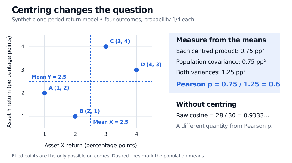
Every scenario places the two assets on the same side of their respective means. Yet correlation is below 1: their centred fluctuations are not proportional. Positive correlation does not require a perfect straight line, and a coefficient of 0.6 does not mean “the returns agree 60% of the time.”
Four equally likely synthetic return pairs in percentage points: A (1,2), B (2,1), C (3,4), D (4,3). Dashed mean lines cross at (2.5,2.5). Every centred product is 0.75 pp squared. Population covariance is 0.75 pp squared, both variances are 1.25 pp squared, and Pearson correlation is 0.6.
Original finite scenario model, not observed market data. The relevant origin for co-movement is the pair of means. All four attained outcomes are filled markers.
For a fixed equal-weight portfolio, the four returns are 1.5, 1.5, 3.5 and 3.5 pp. Its population variance is 1 pp², compared with 1.25 pp² for either asset. The same result follows from portfolio variance: 41(1.25)+41(1.25)+2(21)(21)(0.75)=1. Correlation enters risk through covariance; the weights and individual volatilities still matter. Even perfect negative correlation produces a zero-variance combination only when the exposures offset the centred fluctuations exactly.
A sample uses the same centring, but answers another question
If those four rows instead represent four observed, aligned holding periods, their sample correlation is
Here the centred cross-sum is 3 and both square-sums are 5, giving r=3/5=0.6. Using the usual n−1 divisor, sample covariance is 1 pp² and each sample variance is 5/3 pp². Using n consistently gives 0.75 and 1.25 instead. Either common divisor cancels in the correlation ratio; mixing conventions does not.
The matching answer does not turn a short history into a known population law. In the scenario model, probabilities define the population coefficient exactly. In the empirical reading, r summarises four rows and may estimate an unknown ρ under an appropriate sampling model. Alignment, horizon, selection and serial dependence affect what that estimate can support.
There is also a geometric reading: r is the cosine of the angle between the two mean-centred observation vectors. Omitting centring gives the raw cosine 28/30≈0.9333 for these rows, which is a different quantity. Adding a constant to either series leaves Pearson correlation unchanged; converting pp to decimal returns also leaves it unchanged. Multiplying one series by a negative number reverses its sign. Correlation is symmetric in X,Y and is not a regression slope.
What zero leaves unresolved
Take a separate dimensionless model: U is equally likely to be −1, 0 or 1, and V=U2. Then E[U]=0, E[V]=2/3, and E[UV]=E[U3]=0. Both variances are positive, so their Pearson correlation is zero. Nevertheless, observing U determines V exactly.
Independence implies zero correlation when finite positive variances exist; the converse needs additional structure. It does hold for a jointly Gaussian pair. Having two individually normal marginal distributions is insufficient, and a normality assumption is not required merely to define or calculate Pearson correlation.
Inspect a scatter plot alongside the coefficient. Curvature, an influential extreme observation or a change of regime can matter more than the single summary. Neither a large sample coefficient nor a positive population coefficient establishes causality, stable future diversification or protection in joint tail events. NIST's scatter-plot guidance illustrates why nonlinear patterns and outliers need their own inspection.
For the expectation and covariance calculations, Expectation, Variance and Covariance is available in full with a free signed-in account. Covariance and Correlation develops the population identities and perfect-correlation condition; the full lesson requires membership, with a public preview.
Sources
Dimitri P. Bertsekas and John N. Tsitsiklis, Introduction to Probability, 2nd edition (Athena Scientific, 2008), §4.2, pp. 218–222 — covariance, correlation, affine equality cases and variance of sums.