A scatter plot displays paired observations as points: each row supplies a horizontal coordinate and a vertical coordinate . Its purpose is to expose the shape of the relationship before a single summary number or fitted model compresses it. The NIST graphical guide distinguishes linear patterns, curvature, changing vertical spread and unusual points.
For a risk analyst, two assets' return histories become a cloud of same-period pairs. Each dot answers: “When asset X returned this much, what did asset Y return over that same holding period?” The horizontal axis need not be time, and assigning X to that axis does not make it a cause of Y.
A dot is a matched row
Consider four synthetic observations of simple one-period returns. The displayed numbers are in percentage points: 1 means a 1% return, or 0.01 in decimal notation.
| Matching date | X return (pp) | Y return (pp) | Plotted point |
|---|---|---|---|
| D1 | 1 | 2 | |
| D2 | 2 | 1 | |
| D3 | 3 | 4 | |
| D4 | 4 | 3 |
Both sample means are 2.5 pp. The points generally move upward together, although they do not lie on a straight line. Their sample correlation is
The numerator's centred cross-product sum is 3 pp squared, and each squared-deviation sum is 5 pp squared. The units cancel. Four observations illustrate the calculation; they provide little evidence about a stable future relationship.
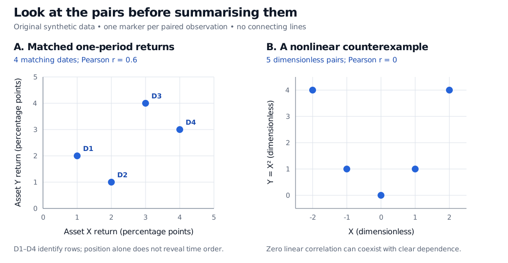
Original synthetic examples. Left: one point per matching date. Right: a separate mathematical counterexample, not return data.
Pair before plotting. Match instrument identifiers, dates, holding periods, time zones and return conventions. Sorting each column separately destroys the pairing and can manufacture an upward pattern. If one return is missing, the row cannot supply the intended point; silently replacing it with zero changes the data. Report which rows were retained and investigate missing data.
A coefficient can miss the shape
The right-hand panel uses and , with dimensionless coordinates. Here , and the centred cross-products sum to zero. Pearson correlation is therefore zero.
Yet knowing X determines Y exactly. If these five pairs are assigned equal probability, X and Y are dependent: for example, Y is zero exactly when X is zero. This is a concrete reason to distinguish correlation from independence. A near-zero coefficient does not rule out an economically relevant curved response. Nor does an unstructured small cloud establish independence or joint normality.
Read the cloud without losing the records
- Direction and shape: look for an upward or downward trend, bends and distinct groups. A straight fitted line can conceal a regime mixture.
- Spread: ask whether vertical dispersion changes with X. A widening cloud can motivate a heteroscedasticity investigation; the picture alone does not establish a complete variance model.
- Unusual observations: identify the dates behind isolated points. An outlier may be an error, a genuine stress event or a different regime. Deleting it automatically can erase the risk being studied.
- Overplotting: several records can occupy the same coordinates. Smaller transparent markers, counts or a disclosed density display can reveal multiplicity. Disclose any jitter because it moves displayed coordinates away from recorded values.
A scatter plot usually hides time order. Permuting whole rows leaves the cloud and correlation unchanged, even though the chronology changes. Use a companion time-series plot or explicit date encodings to investigate temporal structure. Leave points disconnected unless the intended object is a trajectory and the connecting order is stated.
Finally, association supplies neither a causal explanation nor proof that observations are independent across dates. Common market drivers, selection and changing regimes can all shape a return cloud. For the step from paired observations to covariance and a fitted line, see Basic Statistics and Regression, available in full with a free signed-in account; the public page provides a preview.
Sources
- John A. Rice, Mathematical Statistics and Data Analysis, 3rd edition (2007), §10.7, “Exploring Relationships with Scatterplots,” pp. 404–406 — paired-coordinate displays, scale transformations and Pearson correlation as a linear summary. Examples and figure here are original.
- NIST/SEMATECH e-Handbook of Statistical Methods, §1.3.3.26: Scatter Plot — graphical patterns, axis roles, unconnected markers and limits on causal interpretation.