The distinction matters because a completed spreadsheet can conceal an incomplete information set. Replacing blanks with numbers may make a calculation run, while changing the economic question it answers.
Two closes do not reveal three closes
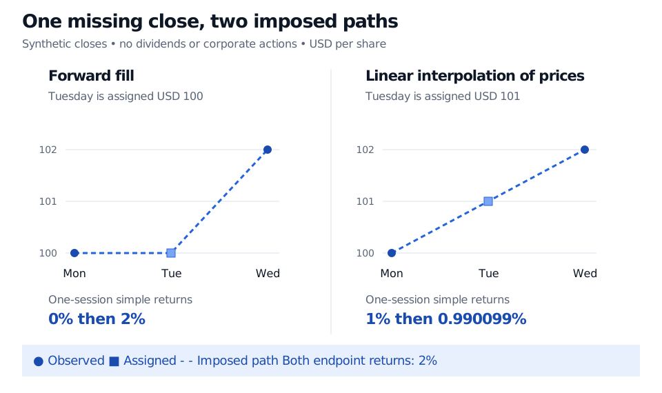
Suppose a synthetic equity dataset contains these closing prices. Tuesday was an intended trading session; assume no dividends or corporate actions during the interval.
| Session | Recorded price, USD per share |
|---|---|
| Monday | 100 |
| Tuesday | Missing |
| Wednesday | 102 |
The Monday-to-Wednesday price return is known:
The two one-session returns are not. If Tuesday's unknown positive price is , they are and . Their compounded return is always
Diagnose what the blank means
Missingness is relative to a defined field, calendar, universe and decision time. Before choosing a treatment, distinguish these cases:
- Unobserved value: an expected market-data message was lost. The economic quantity may exist even though the dataset lacks it.
- Not applicable: no regular-session close was scheduled on an exchange holiday. This is a calendar issue, not necessarily a lost observation. A common calendar across markets needs an explicit interpretation.
- Not yet available: accounts for a completed quarter have not been published. A historical decision must respect the release time.
- Partial information: a measurement is known only to exceed a reporting limit. This is censoring; the bound is information, even though the exact value is unknown.
- An observed zero: a confirmed zero-volume interval is different from an interval for which no volume record arrived.
A security disappearing from a vendor file also does not establish a zero terminal value. Investigate delisting, acquisition, trading halt and identifier changes. Likewise, absence of a trade record does not automatically establish that an order was unfilled. The event log and its coverage determine what can be concluded.
Why the observations are absent
For a simple setup, let be a variable that can be missing, fully observed characteristics, and indicate that was recorded. Three common mechanism labels describe the relationship between values and recording:
| Mechanism | Meaning in this setup | Hypothetical financial example |
|---|---|---|
| Missing completely at random, MCAR | Recording is independent of both and | A genuinely random record-deletion process, independent of all analysed fields |
| Missing at random, MAR | Conditional on , recording does not depend further on | Response probability differs by recorded liquidity group, but not by return within each group |
| Missing not at random, MNAR | Recording still depends on the unobserved after conditioning on | Loss-making trades are less likely to be reported, even within the recorded groups |
These are assumptions about a data-generating and observation process, not descriptions established by seeing a few blanks. MAR does not mean that reported and unreported values have the same marginal distribution. Its plausibility depends on which characteristics are observed. Observed records alone generally cannot distinguish MAR from every possible MNAR alternative.
Treatment follows the target
For predictive work, fit learned imputation rules within the training data available at each decision, then apply them to later data. Compare conclusions under economically defensible alternatives, including leaving a quantity unidentified. A missingness indicator can itself be useful information; it does not by itself remove selection bias.
Sources
- Gelman, A., Carlin, J. B., Stern, H. S., Dunson, D. B., Vehtari, A., and Rubin, D. B. Bayesian Data Analysis, 3rd ed., §§18.1–18.2: observation indicators, missingness mechanisms and multiple imputation.
- Rubin, D. B. (1976). Inference and missing data. Biometrika 63(3), 581–592: the framework for inference with incomplete observations.
- Gelman, A., and Hill, J. (2007). Missing-data imputation, Chapter 25 of Data Analysis Using Regression and Multilevel/Hierarchical Models: practical mechanisms, deletion and imputation.