MNAR means reporting still depends on the missing outcome after conditioning on observed information. Trace selection bias and show what a sensitivity assumption changes.
Missing not at random
Missing not at random (MNAR) means that whether a value is observed still depends on the value that may be missing, after conditioning on the observed information included in the analysis. A return database can therefore understate losses if losing accounts are less likely to submit their results—even when every submitted report is accurate.
MNAR describes a missing-data mechanism relative to an information set. It does not mean that every absent value is bad, that all missingness is deliberate, or that missing values are impossible to analyse.
What would need to be independent?
Let Y be one outcome, X fully observed covariates and R=1 mean that Y is recorded. In this single-outcome setting, missing at random requires
P(R=1∣X,Y)=P(R=1∣X).
MNAR means this equality fails on the model's positive-probability support: knowing Y changes the response probability even after conditioning on X. The relevant idea is conditional independence, rather than the everyday meaning of “random”. Missing completely at random is the stronger condition that recording is independent of both X and Y.
For example, if reporting differs by account size and size is recorded for every account, that dependence alone need not violate MAR. If losses still affect reporting within each size group, the mechanism is MNAR relative to those covariates. Adding a useful observed variable can change the assessment; adding arbitrary columns cannot establish MAR. Gelman and coauthors develop these distinctions in Bayesian Data Analysis, §18.1.
The loss reports that disappear
Consider a synthetic model for one month's account outcomes. Define L=1 for a loss and L=0 for a nonloss; this indicator records occurrence, not loss severity. Assume the full loss probability is 20%. An account submits its outcome with probability 30% after a loss and 90% after a nonloss. There are no other covariates.
The full population loses 20% of the time; submitted reports lose only about 7.69% of the time. An equivalent model ledger has 100 accounts: 6 reported losses, 72 reported nonlosses, 14 unreported losses and 8 unreported nonlosses. These are proportions represented as counts, not a claim that a random sample must reproduce them exactly.
Missing reports are more loss-heavy here, but they are not all losses: their loss probability is 14/22=7/11≈63.64%. Recording absence as a loss would overstate the model's full loss rate. Recording it as a nonloss would understate it. More reports from the same mechanism improve precision about the selected reporting population; they do not remove this sampling bias.
The observed records do not identify the unseen outcomes
The 20%, 30% and 90% probabilities above are supplied assumptions. A researcher normally does not observe the losses in the missing group. Even if an account roster reveals the reporting rate, the available data only reveal whether each account reported and, for reporters, its outcome.
Keep the observed law fixed: 6% of all accounts are reported losses, 72% are reported nonlosses and 22% have unknown outcomes. Let
q=P(L=1∣R=0).
The full loss probability is then
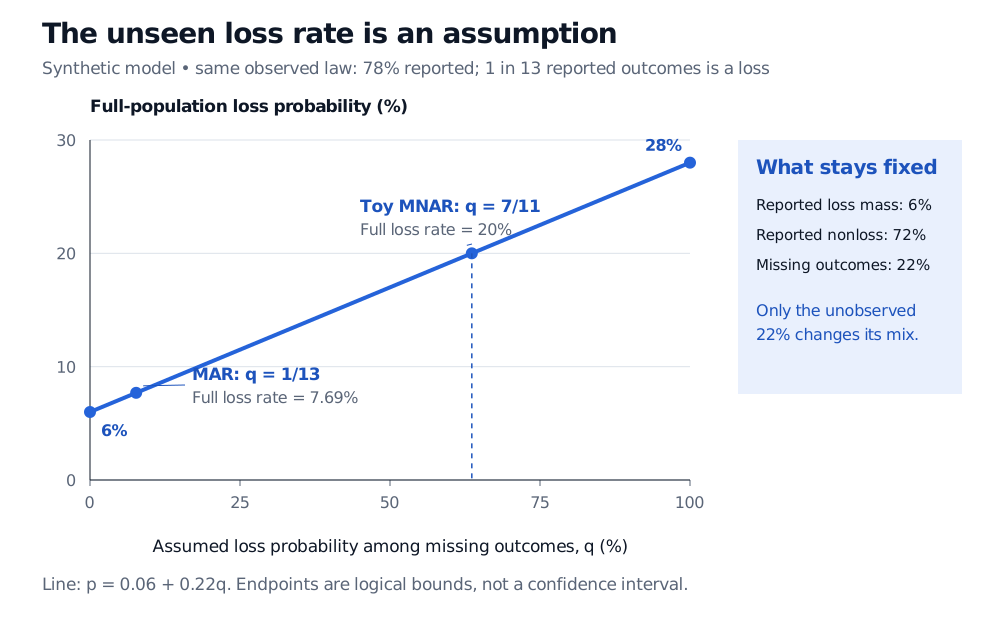
p=P(L=1)=0.06+0.22q.
Every q between zero and one produces the same observed-data law, while changing the full loss probability from 6% to 28%. These are logical bounds with the population reporting proportions treated as known, not a confidence interval. Sampling uncertainty would be an additional issue.
With a fixed 78% reporting rate and reported loss probability 1/13, the full loss probability is 6% plus 22% times q, the unknown loss probability among missing accounts. The MAR point has q equal to 1/13 and full loss probability 7.69%; the toy MNAR point has q equal to 7/11 and full loss probability 20%. Logical endpoints are 6% and 28%.
Original synthetic sensitivity model. The line holds the observed-data law fixed while changing the unobserved group's assumed composition; it does not estimate that composition.
With no covariates, MAR sets q=1/13, matching the reported loss probability. The original MNAR model instead has q=7/11. Both agree on everything observable in this example. This is why an observed-record diagnostic cannot, by itself, certify MAR or determine the MNAR dependence. Collection records or a follow-up audit may supply additional information; the submitted outcomes alone do not.
Make the unverifiable assumption visible
Two useful modelling views expose different assumptions:
A selection model specifies how reporting depends on the full outcome and observed covariates, as the 30% and 90% reporting probabilities did above.
A pattern-mixture model specifies outcome distributions within observed and missing groups, as the parameter q does here.
The National Research Council's chapter on sensitivity analysis develops both views. In this example, a sensitivity analysis can report the consequences of several defensible q values instead of presenting one hidden assumption as a recovered fact. For instance, q=25%, 50% or 75% implies full loss probabilities of 11.5%, 17% or 22.5%. Choosing a plausible range needs knowledge of reporting incentives, operational failures or independent validation data.
Imputation is a way to express a model, not evidence that its missingness assumptions hold. Repeatedly imputing under a MAR model cannot resolve the unidentified dependence illustrated above. An MNAR model can support an analysis, but its extrapolation into missing outcomes must be stated and challenged.
For financial histories, first establish what the missing outcome means. A missing quote, an account that did not report and a security that ceased to exist need different economic treatment. The owned lesson Corporate Actions and Survivorship explains historical inclusion and terminal outcomes, including why neither carrying a last price forever nor assigning zero to every disappearance is a general repair. Its public page is a preview; the full lesson requires membership.
Sources
Gelman, A., Carlin, J. B., Stern, H. S., Dunson, D. B., Vehtari, A. and Rubin, D. B. Bayesian Data Analysis, 3rd ed., §§8.2 and 18.1, especially pp. 449–451: missingness mechanisms, observed information and ignorability. Authors' book page.
National Research Council (2010). The Prevention and Treatment of Missing Data in Clinical Trials, Chapter 4, “Drawing Inferences from Incomplete Data”, and Chapter 5, “Principles and Methods of Sensitivity Analyses”, especially the single-outcome example on pp. 86–88. Chapter 4, Chapter 5. The reporting model and numerical sensitivity illustration here are original financial examples.