Missing completely at random: Definition & Examples

Missing completely at random (MCAR) means that the pattern of missing data is independent of the full data values, including both observed and unobserved values. Losing a return must be unrelated to that return, other returns, and the covariates included in the data model. The claim concerns the mechanism generating missingness; a dataset with scattered blank cells does not establish it.

For a quant researcher, MCAR distinguishes an information loss from a selection effect. A deliberately random record-deletion experiment can satisfy MCAR. An exchange-feed failure during volatile periods needs a different argument: it may disproportionately remove precisely the market conditions whose risk the researcher wants to measure.

What independence requires

Let $D$ contain all potentially observable data values, and let $R$ be the corresponding observation indicators: $R_j=1$ when entry $j$ is observed and $R_j=0$ when it is missing. Here MCAR means, for every possible pattern $r$ and full-data value $d$ in the model,

\mathbb{P}(R=r\mid D=d)=\mathbb{P}(R=r).

This is independence of the whole pattern from the data. Independent coin flips for each record are one way to construct it; independent missingness indicators are not themselves a requirement. For example, randomly choosing one entire batch to delete can be independent of the data even though entries within that batch disappear together. That dependence still matters for uncertainty calculations.

MCAR is stronger than missing at random (MAR), which allows missingness to depend on observed values while excluding further dependence on missing values once the relevant observed information is accounted for. Under missing not at random (MNAR), that remaining dependence on missing values is present. The variables included in the model matter when making these distinctions.

A random deletion can reverse the reported mean

Consider six synthetic one-period strategy returns, measured in percentage points:

(-3,-1,0,1,2,7),\qquad \mu=\frac{-3-1+0+1+2+7}{6}=1.

Retain each record independently with probability $1/2$ , without consulting any value or covariate. This stipulated mechanism is MCAR. One possible retained set is the first three returns. Its sample mean is

\bar y_{\mathrm{obs}}=\frac{-3-1+0}{3}=-\frac43 \quad\text{percentage points}.

The sign changed despite completely random deletion. MCAR does not guarantee that a realised retained sample matches the original population.

Six synthetic returns have full mean 1 percentage point. Retaining the first three gives mean minus 4/3 percentage points. Attainable retained-mean ranges shrink with retained count; each count has expected mean 1 percentage point.

Original finite-population example. Filled range endpoints are attainable extremes, not confidence intervals; the blue dots show expected retained means conditional on the retained count.

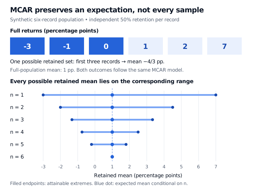
There are $2^6=64$ equally likely observation patterns. The empty pattern has probability $1/64$ and its mean is undefined. Conditional on retaining at least one record, each of the other 63 patterns has probability $1/63$ . Averaging their means gives

\mathbb{E}[\bar y_{\mathrm{obs}}\mid N_{\mathrm{obs}}>0]=1 \quad\text{percentage point}.

Why? Conditional on retaining $n>0$ records, every size- $n$ subset is equally likely. Each original return enters a proportion $n/6$ of those subsets. Taking the average of their means therefore gives $(1/n)(n/6)\sum_i y_i=1$ . Averaging over positive retained counts preserves that result. This exact enumeration needs no large-sample approximation.

What the assumption buys—and leaves unresolved

For independent, identically distributed observations with finite variance, value-independent retention preserves the outcome distribution among retained observations. A retained-sample mean, conditional on a positive retained count, targets the same population mean. Complete-case analysis can consequently avoid bias caused by value-dependent deletion under MCAR. This does not make every estimator unbiased or repair a biased original sampling frame.

Deletion still discards information. A smaller retained sample generally gives less precise estimates; correlated data or clustered deletions require their own uncertainty treatment. Replacing blanks with the observed mean does not restore the lost observations or their variability.

In real market data, inspect collection logs, outage timing, liquidity and instrument coverage. An association between missingness and observed covariates can contradict MCAR. An absence of detectable association cannot prove independence from unobserved returns. Neither a missingness plot nor a reassuring retained mean settles the mechanism. State the assumption and examine how conclusions change under plausible alternatives.

The Point-in-Time Data lesson develops a related operational discipline: preserve why a value is missing, its availability time, and the permitted fallback. Its public page is a preview; the full lesson requires membership.

Sources

Hastie, T., Tibshirani, R. and Friedman, J. (2009), The Elements of Statistical Learning, second edition, §9.6, “Missing Data,” especially equation (9.32).
Seaman, S., Galati, J., Jackson, D. and Carlin, J. (2013), “What Is Meant by ‘Missing at Random’?”, Statistical Science 28(2), 257–268, §2, especially Definition 5 (everywhere MCAR).
University of Melbourne Statistical Consulting Centre, “Missing data”, discussion of mechanisms, complete cases and information loss.

What independence requires

A random deletion can reverse the reported mean

What the assumption buys—and leaves unresolved

Sources

Related terms

Independence

Missing at random

Missing data

Missing not at random