MAR makes missingness independent of unseen values conditional on observed information. A liquidity example shows why reported returns can still be biased and how weighting works.
Missing at random
Missing at random (MAR) means that, after conditioning on the relevant observed information, the probability that a value is missing does not depend on that value's unobserved magnitude. Missing returns can therefore be more common in some kinds of securities than others. The key assumption is that the observed information accounts for the remaining selection within those groups.
The word “random” is easy to misread. MAR does not say that the available records are a representative sample, or that missing and reported returns have the same overall average.
What information makes missingness explainable?
Let Y be a one-period return, X a set of covariates recorded for every security, and R an indicator equal to 1 when Y is observed and 0 when it is missing. In this single-outcome setting, MAR is the conditional independence assumption
P(R=1∣X,Y)=P(R=1∣X)=s(X).
Holding X fixed, learning the return itself would not change the observation probability. The conditioning set matters: MAR given liquidity and exchange need not imply MAR given exchange alone. A covariate that is also missing cannot simply be treated as fully observed.
Missing completely at random (MCAR) is stronger: observation is independent of both X and Y. If missingness still depends on unobserved returns after conditioning on X, the mechanism is missing not at random (MNAR). These labels concern an assumed data-generating mechanism, not a pattern that spreadsheet blanks reveal by themselves. The general multivariable MAR definition allows dependence on whichever values are observed for the particular missingness pattern; the equation above is its useful special case with one incomplete outcome.
A return database that favours liquid securities
Consider an original synthetic population of security-period records. Liquidity class X is available for all records. Half are liquid, half illiquid. Returns Y are measured in percentage points (pp): a value of 1 means a 1% return.
Liquidity class
Possible returns, equally likely within class
Mean return
Probability return is observed
Liquid
1 pp, 3 pp
2 pp
90%
Illiquid
−3 pp, −1 pp
−2 pp
50%
Assume that observation is independent of the return within each liquidity class. The two liquid outcomes each have observation probability 90%; the two illiquid outcomes each have probability 50%. This is MAR given liquidity. It is not MCAR because observation rates differ by liquidity.
The population expected return is 0.5(2)+0.5(−2)=0 pp. But 70% of records are observed:
P(R=1)=0.5(0.9)+0.5(0.5)=0.7.
Liquid records supply 0.45/0.7=9/14 of the observed distribution, rather than one half. The reported-return mean is
E[Y∣R=1]=0.70.5(0.9)(2)+0.5(0.5)(−2)=74 pp≈0.5714 pp.
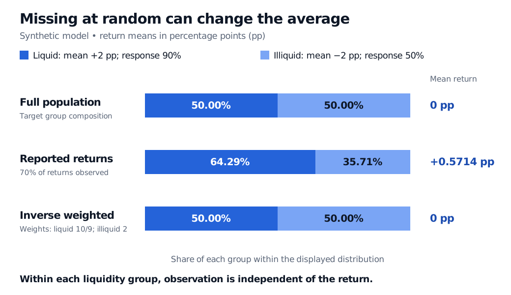
Synthetic MAR example: liquid and illiquid records each make up 50% of the full population, with group means plus 2 and minus 2 pp. Reporting rates of 90% and 50% change the observed mix to 64.29% liquid and 35.71% illiquid and the mean to plus 0.5714 pp. Inverse response weighting restores the 50/50 mix and mean zero.
Original synthetic model. Bars show group shares within each displayed distribution, not counts. Inverse weights use the stipulated observation probabilities; the corrected mean is a population calculation.
The upward shift is sampling bias in the unadjusted mean. It appears even though no return is selectively suppressed within its liquidity class. MAR allows the group composition to change.
Recover the population mix, with assumptions
Under MAR and positive observation probabilities, the reported returns within each liquidity class have the same distribution as that class's full returns. One adjustment is to estimate each class mean and average those means using the full population's class proportions. Here that gives 0.5(2)+0.5(−2)=0 pp again.
Another is inverse response weighting. A reported liquid record receives weight 1/0.9=10/9 and an illiquid record weight 1/0.5=2. The population identity is
E[s(X)RY]=E[s(X)YE[R∣X,Y]]=E[Y].
For the example, the weighted mean contributions are 0.45(2)/0.9=1 pp and 0.25(−2)/0.5=−1 pp. Their sum is zero; the weighted probability mass is 0.45/0.9+0.25/0.5=1.
This needs positivity: s(x)>0 for every population group of interest. If an entire class never reports, weighting cannot recover its return distribution. Very small observation probabilities produce large weights and unstable estimates. In applications, estimated probabilities also need an adequate response model and appropriate uncertainty calculations. A finite-sample ratio of weighted sums need not be exactly unbiased merely because this population identity holds.
MAR can also support likelihood methods or multiple imputation. Their validity depends on the models and inferential conditions; it does not justify filling blanks with zero or using an unconditional average. Ignoring the missingness mechanism in a likelihood analysis requires additional conditions such as distinct data-model and missingness-model parameters; Bayesian ignorability also involves the prior specification. It still requires analysing the observed information appropriately. Rubin's original paper sets out this distinction.
What the available records cannot establish
Because X and R are known for every record, a researcher can examine how observation rates vary by liquidity. That helps diagnose a claim of MCAR and design a response model. It cannot establish that the unseen returns have the same within-class distribution as the reported ones. A mechanism that also suppresses unusually poor unreported returns could generate the same observed records.
For real research, document the data-collection process, collect useful auxiliary information and check sensitivity to plausible departures from MAR. “Liquidity is recorded” is evidence that an adjustment is possible; “liquidity explains all remaining outcome-dependent missingness” is an assumption requiring justification. Seaman and coauthors distinguish these missingness assumptions from the conditions needed for valid inference.
The owned Conditional Expectation lesson develops the tower property used in the weighting identity. Point-in-Time Data explains how to record missingness reasons, staleness and permitted fallbacks in a research dataset. Both have public previews; full lessons require membership.
Sources
Gelman, Carlin, Stern, Dunson, Vehtari and Rubin, Bayesian Data Analysis, 3rd ed., §8.2, “Data-collection models and ignorability.”
Wooldridge, Econometric Analysis of Cross Section and Panel Data, Chapter 17, pp. 587–589, equations 17.64–17.65: selection on observables and inverse probability weighting.