Multivariate normal distribution: Definition & Examples

A multivariate normal distribution is a joint probability law for a vector in which every fixed linear combination of its components is normally distributed, allowing a constant as a zero-variance normal. It is also called a joint Gaussian law. In portfolio modelling, this assumption does more than assign each asset a bell curve: it makes every fixed linear portfolio return normal, with a distribution determined by the mean vector and covariance matrix.

Write $\mathbf{R}\sim\mathcal{N}_d(\boldsymbol\mu,\Sigma)$ . Then, for every fixed vector $\mathbf{a}\in\mathbb{R}^d$ ,

\mathbf{a}^\top\mathbf{R}\sim\mathcal{N}\!\left(\mathbf{a}^\top\boldsymbol\mu,\;\mathbf{a}^\top\Sigma\mathbf{a}\right).

Here

\boldsymbol\mu=\mathbb{E}\mathbf{R}]

, and the [covariance matrix has entries

\Sigma_{ij}=\text{Cov}(R_i,R_j)

. Its diagonal contains variances; its off-diagonal entries contain covariances. The second argument of

\mathcal{N}

is variance, not standard deviation. The corresponding univariate normal distribution is the useful starting point for reading the formulas.

Two assets, one portfolio distribution

Consider a hypothetical one-period simple-return model, in decimal return units, under a stipulated physical probability law:

\boldsymbol\mu=\begin{pmatrix}0.01\\0.02\end{pmatrix}, \qquad \Sigma=\begin{pmatrix}0.0004&0.0003\\0.0003&0.0009\end{pmatrix}.

Asset 1 has mean return 1% and standard deviation 2 percentage points; asset 2 has mean return 2% and standard deviation 3 percentage points. Their correlation is

\rho=\frac{0.0003}{0.02\times0.03}=0.5.

For a fully invested portfolio with equal period-start weights, no cash flows and no trading within the period,

R_P=0.5R_1+0.5R_2

. Its mean is

0.015

, and its portfolio variance is

\begin{aligned} \sigma_P^2 &=0.5^2(0.0004)+0.5^2(0.0009) +2(0.5)(0.5)(0.0003)\\ &=0.000475. \end{aligned}

Thus

R_P\sim\mathcal{N}(0.015,0.000475)

, with standard deviation

\sqrt{0.000475}\approx0.0217945

, or 2.17945 percentage points. Standardising gives

\mathbb{P}(R_P<0) =\Phi\!\left(\frac{-0.015}{\sqrt{0.000475}}\right) \approx0.245649,

where

\Phi

is the standard normal cumulative distribution function. The model therefore assigns a 24.56% probability of a negative portfolio return.

The mean and variance calculations require finite second moments, not normality. Joint normality supplies the extra step from two moments to the whole portfolio distribution. With a different joint law having the same mean vector and covariance matrix, the loss probability need not be 24.56%. A nonlinear option portfolio also need not have normal P&L even when its underlying risk-factor changes are jointly Gaussian.

What observing one asset tells you

The Gaussian conditional distribution is particularly tractable. For this two-asset model,

R_2\mid R_1=r \sim\mathcal{N}\!\left( 0.02+\frac{0.0003}{0.0004}(r-0.01),\; 0.0009-\frac{0.0003^2}{0.0004} \right).

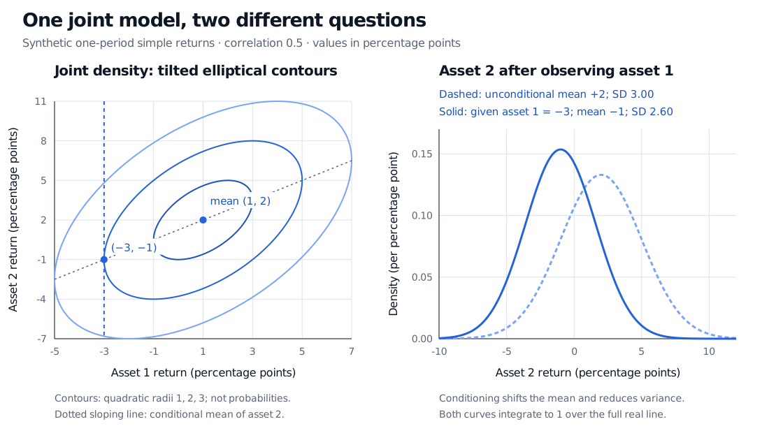
If asset 1 returns $-3\%$ , the conditional mean of asset 2 becomes

0.02+0.75(-0.03-0.01)=-0.01,

and the conditional variance is $0.000675$ . Thus

R_2\mid R_1=-0.03\sim\mathcal{N}(-0.01,0.000675).

Its conditional standard deviation is about 2.59808 percentage points, down from 3. The conditional loss probability is about 64.98%, compared with 25.25% before observing asset 1. Positive correlation has shifted the mean downward enough to make a loss more likely, even though remaining variance is smaller.

Joint Gaussian return contours for asset 1 mean 1% and standard deviation 2 percentage points, asset 2 mean 2% and standard deviation 3 percentage points, with correlation 0.5. Observing asset 1 at minus 3% gives asset 2 conditional mean minus 1% and standard deviation 2.60 percentage points, compared with unconditional mean 2% and standard deviation 3 percentage points.

Original synthetic one-period model. Left: equal-density ellipses at quadratic radii 1, 2 and 3, with the conditional-mean line and the observed asset 1 return. These contour labels are not enclosed probability levels. Right: unconditional and conditional asset 2 densities; the finite plot windows do not truncate either law.

Conditioning on an exact value of a continuous variable is understood through a conditional density, rather than dividing by $\mathbb{P}(R_1=-0.03)$ , which is zero. This is a same-period conditional relationship, not a causal claim or automatically a forecast available before that period begins.

A Gaussian model keeps the conditional variance constant across observed values of asset 1. A more extreme observation changes the conditional mean but does not itself increase this residual variance. That is a meaningful restriction when modelling stress. It does not say that losses in correlated assets cannot become more likely after a bad observation; the calculation above shows they can.

A joint law is stronger than normal marginals

Normality of each asset separately does not establish joint normality. A compact counterexample uses $Z\sim\mathcal{N}(0,1)$ and an independent fair sign $B\in\{-1,1\}$ . Set $X=Z$ and $Y=BZ$ . Both marginals are standard normal, and

\text{Cov}(X,Y)=\mathbb{E}[BZ^2]=0.

Yet

\lvert X\rvert=\lvert Y\rvert

always, so the variables are dependent. Furthermore,

X+Y

equals zero with probability

1/2

and has positive variance; it cannot be a nondegenerate normal, which has no point masses. The vector is therefore not jointly normal. This illustration is also used in Patrick Breheny's university notes cited below.

Within a jointly Gaussian vector, zero covariance between two components does imply independence. That implication depends on the joint Gaussian assumption; two normal-looking histograms and a near-zero sample correlation do not establish it.

Valid covariance does not always mean a density

A Gaussian covariance matrix must be symmetric and positive semidefinite:

\mathbf{a}^\top\Sigma\mathbf{a}\ge0

for every

\mathbf{a}

, because no linear combination can have negative variance. An equivalent construction is

\mathbf{R}=\boldsymbol\mu+A\mathbf{Z},\qquad \Sigma=AA^\top,

where $\mathbf{Z}$ has independent standard normal components. A Cholesky decomposition provides such a factor for a positive-definite covariance matrix; a rank-aware factorisation also handles singular cases.

When

\Sigma

is positive definite, the full

d

-dimensional probability density is

f(\mathbf{r})= \frac{\exp\!\left[-\frac12(\mathbf{r}-\boldsymbol\mu)^\top \Sigma^{-1}(\mathbf{r}-\boldsymbol\mu)\right]} {(2\pi)^{d/2}\lvert\Sigma\rvert^{1/2}}.

For the example,

\det\Sigma=0.00000027>0

and both variances are positive, so this density exists. But singular positive-semidefinite covariance still defines a valid Gaussian law. If instead

R_1=0.01+0.02Z

and

R_2=0.02+0.03Z

share one standard normal shock, their covariance is

0.0006

and the covariance determinant is zero. All outcomes lie on a line. There is no full two-dimensional density, and the inverse/determinant formula above is unavailable; the distribution itself remains valid. The linear combination

1.5R_1-R_2=-0.005

is deterministic.

Finally, a nondegenerate normal simple-return model has support below

-100\%

. That is incompatible with the literal simple return of an unlevered limited-liability asset, whose loss is bounded below by

-100\%

. Treat it as an approximation over a stated horizon and range. Gaussian log returns avoid that price-bound problem after exponentiation, but simple returns then become lognormal minus one, and weighted simple portfolio returns do not automatically remain Gaussian. Model convenience does not settle tail behaviour, stability of covariance estimates or model risk.

For a longer derivation of bivariate conditioning and the portfolio closure property, see Multivariate Normal Distribution in the Mathematics Library (membership for the full lesson; public preview).

Sources

Damien Lamberton and Bernard Lapeyre, Introduction to Stochastic Calculus Applied to Finance, 2nd edition, 2008, Appendix A.1.3: Gaussian vectors and the Gaussian independence theorem.
John C. Hull, Options, Futures, and Other Derivatives, 9th Global Edition, 2018, §§22.4 and 22.7: linear Gaussian portfolio models and distributional limitations.
Merlise A. Clyde, Duke University, Multivariate Normal Theory: linear transformations, including positive-semidefinite covariance.
Patrick Breheny, University of Iowa, Multivariate normal distribution, BIOS 7110, slides 6–8, 12–14 and 20–22: singular distributions, the fair-sign counterexample, linear transformations and Gaussian conditioning.

Two assets, one portfolio distribution

What observing one asset tells you

A joint law is stronger than normal marginals

Valid covariance does not always mean a density

Sources

Related terms

Conditional distribution

Correlation

Independence

Model risk

Normal distribution

Portfolio variance

Positive definite matrix

Positive semidefinite matrix

Probability density function