Fama-Bliss Forward Rate Regressions: Definition & Examples

Fama–Bliss forward rate regressions use the gap between a one-year forward rate and today’s one-year spot rate to forecast either a bond’s excess return or a change in the one-year spot rate. The two targets help explain what a steep yield curve is signalling. A high forward can coincide with a higher expected return on the longer bond even if investors expect little near-term change in the short rate. Fama’s prize lecture, equations (10)–(11)

A two-year bond turns the spread into a break-even test

Use continuously compounded rates throughout. At date

t

, let

y_t^{(n)}

be the annualised yield of an

n

-year zero-coupon bond and

P_t^{(n)}

its price per unit of face value. The forward for the year ending at

t+n

comes from adjacent discount factors. Write the forward and the predictor as

f_t^{(n)}=\log\frac{P_t^{(n-1)}}{P_t^{(n)}}=ny_t^{(n)}-(n-1)y_t^{(n-1)}, \qquad s_t^{(n)}=f_t^{(n)}-y_t^{(1)}.

Suppose the one- and two-year spot rates today are 3.0% and 3.5%. The one-year forward for the second year is

2(3.5\%)-3.0\%=4.0\%

, so the forward–spot spread is 1.0 percentage point.

One year later, suppose the one-year spot rate is 3.6%. The original two-year zero now has one year left. Its log holding-period return is

\log(e^{-0.036}/e^{-0.070})=3.4\%

. The one-year zero bought at the same time matured and earned 3.0% in logs, so the longer bond earned 0.4% in excess log return. At a realised one-year rate of 4.0%, the two holdings would have broken even against each other. A higher realised rate would have cut the resale price enough for the longer bond to underperform.

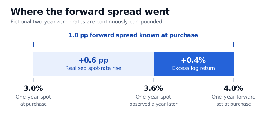
\underbrace{f_t^{(2)}-y_t^{(1)}}_{\text{known at purchase}} = \underbrace{y_{t+1}^{(1)}-y_t^{(1)}}_{\text{realised spot-rate change}} + \underbrace{f_t^{(2)}-y_{t+1}^{(1)}}_{\text{realised excess log return}}.

The fictional 1.0 percentage point gap from today's 3.0% one-year spot to today's 4.0% forward splits at the 3.6% spot observed one year later. The spot rises 0.6 percentage points and the two-year zero earns 0.4% in excess log return.

The forward and current spot rate are both known at purchase. The location of the split becomes known when the new one-year spot rate is observed.

The SelfMadeQuant lesson derives forwards from bond prices and works through how a realised rate above or below a forward affects relative bond performance. It uses semiannual compounding. Spot Rates, Forward Rates, and the Term Structure Slope (public preview, full lesson for members)

What goes on the left-hand side?

Bond return. Buy the $n$ -year zero, sell it one year later with $n-1$ years left, and subtract the log return locked in by the initial one-year zero. The excess log return is $\log(P_{t+1}^{(n-1)}/P_t^{(n)})-y_t^{(1)}$ . Regress it on $s_t^{(n)}$ . A positive slope means wider spreads have historically been associated with larger subsequent excess returns.
Spot-rate change. Regress $y_{t+n-1}^{(1)}-y_t^{(1)}$ on the same spread. This target waits for the quoted forward interval to begin. A five-year zero helps construct the one-year forward starting in four years. The return test still waits one year, while the spot-rate test waits four.

For the two-year case, fitting both regressions by ordinary least squares with an intercept on the same dates gives slopes that sum to one, by the identity above. Under a constant expected log excess return, the return slope would be zero and the spot-change slope one. The pure expectations hypothesis benchmark in logs also sets the expected excess return itself to zero. For longer bonds, the one-year return depends on the yield of the bond with

n-1

years left at resale. The four-year-ahead change in the one-year spot rate is a different outcome, so the two slopes need not sum to one. Fama’s prize lecture

Fama and Bliss’s 1987 study used nominal U.S. Treasury maturities from one to five years, with the one-year bond as the return benchmark for the two- through five-year bonds. The original return regressions are reported for 1965–1985. Forward spreads helped forecast excess returns, while the one-year-ahead change in the one-year spot rate was hard to predict. Forwards starting two to four years ahead had more explanatory power for the corresponding spot-rate changes. Here a time-varying term premium means the expected one-year excess return on a longer bond changes over time. Fama and Bliss (1987), Chen and Pakoš, discussion of Table 1, Fama (1990), introduction

Using the spread as a forecast benchmark

On each forecast date, build the predictor from a single zero curve available at that time. Reprice the aged bond from the curve available at the end of the holding period. For an expanding-window forecast, fit the coefficients only on rows whose outcomes are already observable at the forecast timestamp. A January row predicting a twelve-month return is unavailable for training in February, even though its predictor was known in January. The same rule applies to spot-change labels at longer horizons. Compare the return forecast against a historical-mean forecast estimated using the same information, and the spot-change forecast against an unchanged-rate forecast. Look-ahead bias

Adjacent monthly observations of one-year returns share eleven months of exposure. The forecast errors can therefore be serially dependent. For inference use a dependence-aware covariance estimate such as Newey–West standard errors, with lag choices that account for the overlap and any additional dependence. Longer spot-change horizons overlap even more. Non-overlapping samples can help check sensitivity, at the cost of fewer observations. Cochrane and Piazzesi (2005), §I.C

The Cochrane–Piazzesi factor uses several forwards to forecast the same kind of excess return. Campbell–Shiller yield curve regressions use a long-minus-short yield spread and ask different questions about subsequent yields. An in-sample result can be evidence against a constant-premium benchmark without providing a dependable forecast for allocation. Thornton and Valente found that forward-based models did not deliver systematic gains over their no-predictability benchmark in an out-of-sample allocation test. Cochrane and Piazzesi (2005), §I.D, Thornton and Valente (2012)

Sources

Fama, E. F., and R. R. Bliss (1987). The Information in Long-Maturity Forward Rates. American Economic Review, 77(4), 680–692.
Chen, H., and M. Pakoš (2008). Asset Pricing with Uncertainty About the Long Run, discussion following equation (63).
Fama, E. F. (1990). Term-Structure Forecasts of Interest Rates, Inflation, and Real Returns. Journal of Monetary Economics, 25(1), 59–76.
Fama, E. F. (2013). Two Pillars of Asset Pricing, “Predictive Regressions,” equations (10)–(11).
Cochrane, J. H., and M. Piazzesi (2005). Bond Risk Premia. American Economic Review, 95(1), 138–160.
Thornton, D. L., and G. Valente (2012). Out-of-Sample Predictions of Bond Excess Returns and Forward Rates: An Asset Allocation Perspective. Federal Reserve Bank of St. Louis working paper, February 2012 version.

A two-year bond turns the spread into a break-even test

What goes on the left-hand side?

Using the spread as a forecast benchmark

Sources

Related terms

Campbell-Shiller Yield Curve Regressions

Cochrane–Piazzesi bond return factor

Discount factor

Forward interest rate

Holding-period return

Look-ahead bias

Ordinary least squares

Spot interest rate

Yield curve

Zero-coupon bond