Cochrane–Piazzesi bond return factor: Definition & Examples

The Cochrane–Piazzesi bond return factor is a fitted combination of today's one-year forward interest rates that forecasts the next year's excess returns on US Treasury bonds. It turns the shape of the yield curve into one signal, then scales that signal by maturity. Two curves can have the same five-year minus one-year yield spread and imply different return forecasts. Cochrane and Piazzesi, §I

The return you are forecasting

Buy an

n

-year Treasury zero-coupon bond today and sell it a year later, when it has

n-1

years left. Compare its log holding-period return with what a one-year Treasury zero bought on the same day earns by maturing. With

P_t^{(n)}

denoting the price per dollar of face value and

y_t^{(n)}=-\log P_t^{(n)}/n

the continuously compounded zero yield,

rx_{t+1}^{(n)}=\log\frac{P_{t+1}^{(n-1)}}{P_t^{(n)}}-y_t^{(1)},\qquad n=2,3,4,5.

The one-year zero sets the benchmark. The longer bond's sale price is unknown when the signal is computed. Cochrane and Piazzesi, §I.A

From the curve to one number

The input $f_t^{(n)}$ is the one-year rate for the period ending $n$ years from today. For example, $f_t^{(3)}$ covers year two to year three. From today's discount factors,

f_t^{(n)}=\log\frac{P_t^{(n-1)}}{P_t^{(n)}}=n y_t^{(n)}-(n-1)y_t^{(n-1)},\qquad n=2,3,4,5.

The first input is

f_t^{(1)}=y_t^{(1)}

. Fit a regression of the average of the four future excess returns on these five inputs and an intercept. The fitted value

x_t

is the factor. In a second regression for each maturity, estimate how much the bond's expected excess return moves with the common factor.

x_t=\hat\gamma_0+\sum_{j=1}^{5}\hat\gamma_j f_t^{(j)}, \qquad \widehat{rx}_{t+1}^{(n)}=\hat b_n x_t.

The historical forward-rate coefficients form a tent. The middle gets the largest positive weight and the ends get negative weights. This shape comes from fitting later returns. Principal components of yields, such as level, slope and curvature, are selected to explain variation in yields. A small movement in yields can carry information about returns even when it contributes little to overall yield variance. Cochrane and Piazzesi, Table 1 · §II.A

Same spread, different scores

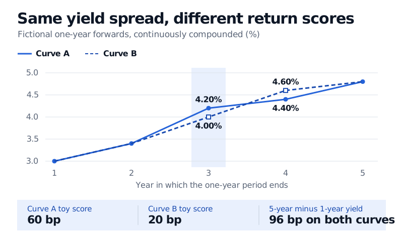
Suppose the one-year inputs for years one through five are 3.00%, 3.40%, 4.20%, 4.40% and 4.80%, all continuously compounded. For a fictional intercept of zero and weights $(-1,0,2,0,-1)$ , the toy score is

-3.00\%+2(4.20\%)-4.80\%=0.60\%=60\ \text{bp}.

Now shift 20 bp from the year-three forward to the year-four forward. The five-year zero yield is the average of the five one-year inputs, so it stays at 3.96% and the five-year minus one-year yield spread stays at 96 bp. The toy score weights the year-three forward by two and the year-four forward by zero, so it falls by 40 bp to 20 bp. These are illustrative weights and scores. A realised return still depends on the sale price in a year.

Two fictional forward curves both give a 96 bp five-year minus one-year yield spread. From curve A to B, the year-three forward falls from 4.20% to 4.00% and the year-four forward rises from 4.40% to 4.60%. The toy score falls from 60 to 20 bp.

Moving 20 bp from the year-three forward to the year-four forward preserves the five-year zero yield. Only the year-three move affects these illustrative scores.

What the evidence supports

Using Fama–Bliss zero-coupon data for US Treasuries from 1964 to 2003, the factor based on the current curve explained 35% of the in-sample variation in the average annual log excess return. The individual one-factor fits had

R^2

values from 31% to 37%, versus 9% to 18% for the Fama–Bliss benchmark, which uses the corresponding forward rate minus the one-year yield for each bond. The authors rejected the exact one-factor restriction with contemporaneous inputs even though it captured most of the variation in fitted expected returns. Cochrane and Piazzesi, Tables 1–2 and §V

Monthly forecast dates produce overlapping annual return windows. The original paper used overlap-adjusted standard errors and checked how its tests behaved in small samples. For an out-of-sample comparison, avoid look-ahead bias by fitting the weights only on returns whose holding periods have ended. Use the curve data available at each forecast date and evaluate both models on the same dates. Cochrane and Piazzesi, §I.C · Appendix, §B.3

The Zero-Coupon Bonds, Market Rates, Swaps, and Conventions lesson derives the forward rate from adjacent discount factors. The preview is public and the full lesson requires membership.

Sources

Cochrane and Piazzesi (2005), Bond Risk Premia. American Economic Review, 95(1), 138–160. Sections I–II and V cover the regressions, curve factors and tests of the one-factor model.
Cochrane and Piazzesi, Appendix to Bond Risk Premia. Sections A.1–A.3 and B.3 cover the benchmark regressions and historical real-time forecasts.

The return you are forecasting

From the curve to one number

Same spread, different scores

What the evidence supports

Sources

Related terms

Excess return

Fama-Bliss Forward Rate Regressions

Forward interest rate

Linear regression

Look-ahead bias

Yield curve

Zero-coupon bond