Campbell–Shiller yield curve regressions test whether today's long-minus-short spread on the yield curve predicts subsequent rate changes as the expectations hypothesis implies. One regression follows a long bond as it ages. The other follows a series of short rates. For a rates analyst, the distinction matters because a steep curve can precede a decline in the first yield and increases in the second set of rates. Campbell and Shiller (1991), §§2–3
Follow the long bond as it ages
Let be the annualised, continuously compounded zero-coupon yield at time for maturity . Use years for and , with , and set . The long-yield regression is
The later observation comes from the point of the curve because the original bond has aged by years. The maturity factor converts today's spread into the yield rise that would make the long bond's holding-period log return equal to the short bond's. The two sides of the regression can therefore both be expressed in basis points of annualised yield. With rational expectations and a constant term premium for the maturity pair, the slope restriction is . The intercept absorbs a constant premium. Campbell and Shiller (1991), §2, eq. (2)
In a synthetic example, today's five-year and one-year yields are 4.00% and 3.00%. The 100 bp spread is scaled by to +25 bp. A unit slope and zero intercept give a benchmark of 4.25% for the same bond's four-year yield next year. If that yield comes in at 3.80%, the realised change is −20 bp and the realised-minus-benchmark error is −45 bp. This is one forecast error. Estimating the slope requires a time series of such observations.
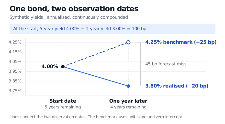
The same zero-coupon bond is observed at the start and one year later. The benchmark assumes a unit slope and a zero intercept.
The return interpretation follows from log prices. Per unit face value, the log price is . The excess log return over years is . In this example the −45 bp yield error translates into +180 bp of excess log return over the year. If you regress excess log returns directly on the spread, the constant-premium null is a zero slope. Andreasen, Jørgensen and Meldrum, §2.1
Follow successive short rates
When is an integer, take the realised -year yields observed at the start of each successive -year block. The short-rate regression uses their average, including today's yield, minus today's yield.
This target is equivalent to a weighted sum of successive short-rate changes. An early rise receives more weight because it enters more of the later yield levels in the average. Here the predictor is the unscaled spread. The constant-premium expectations hypothesis again implies a slope of one. In the five-year example the target requires the one-year yields at each annual observation through year four. The four-year yield observed next year belongs to the other regression. Campbell and Shiller (1991), §2, eq. (3)
Read the slope with its horizon
In Campbell and Shiller's U.S. Treasury sample from January 1952 to February 1987, the long-yield regression slopes were predominantly negative. The short-rate slopes were mostly positive and tended to be closer to one for longer maturities of the long bond. Predicting the direction of the short-rate target is a weaker result than getting a slope of one. Time-varying premia could help explain why the two tests perform differently. The regression slopes alone leave the contribution of premia unidentified. Campbell and Shiller (1991), Tables 1–2 and §4
With monthly observations, adjacent rows can share much of the future rate window, especially in the short-rate regression. Use inference that accounts for overlapping errors and changing error variance. With long horizons relative to the sample, even adjusted standard errors can be unreliable. Campbell and Shiller (1991), §§2–3
Sources
- John Y. Campbell and Robert J. Shiller (1991), Yield Spreads and Interest Rate Movements: A Bird's Eye View, The Review of Economic Studies, 58(3), 495–514.
- Martin M. Andreasen, Kasper Jørgensen and Andrew Meldrum, Bond Risk Premiums at the Zero Lower Bound, §2.1.