A gateway to rates of change, local approximation and optimisation, with a trading-cost example separating average cost from marginal cost.
Differential calculus
Differential calculus is the branch of calculus that studies rates of change, local approximation and the behaviour of functions through their derivatives. In finance, it turns “what happens if this input moves?” into a measurable sensitivity: the extra cost of a larger trade, a bond price's response to yield, or an option price's response to its underlying.
when this finite limit exists. The quotient measures average change over a step; its limit measures the slope at a point. Multiplying that slope by a small input move gives the local approximation
f(a+h)≈f(a)+f′(a)h.
The units matter: an output measured in USD and an input measured in shares give a derivative measured in USD per share.
A trading-cost curve has three different readings
Suppose an execution desk uses the synthetic cost model
C(q)=10+0.1q+0.001q2,q≥0,
where q is the numerical quantity in shares and C(q) is the numerical cost in USD. The coefficients correspond to USD 0.1 per share and USD 0.001 per share squared. The USD 10 baseline cost is incurred even when q=0; it is not a fee triggered only by placing an order. Treat quantity as continuous for the sensitivity calculation, then compare whole-share changes explicitly.
At q=50:
Question
Calculation
Answer
What is the total cost?
C(50)
USD 17.50
What is the cost per share on average?
C(50)/50
USD 0.35 per share
How fast is cost rising here?
C′(50)=0.1+0.002(50)
USD 0.20 per share
What does one additional share actually cost?
C(51)−C(50)
USD 0.201
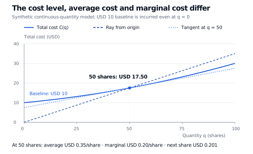
Average cost spreads the baseline across the order. Marginal cost differentiates the cost function, so the constant baseline drops out. The two answer different questions.
Synthetic cost curve: total cost at 50 shares is USD 17.50; the origin ray has slope USD 0.35 per share and the tangent has slope USD 0.20 per share.
Original synthetic model. The origin ray measures average cost; the tangent measures marginal cost. The curve starts at USD 10 because the baseline is incurred at zero quantity.
For this quadratic model, the exact increment is
C(50+h)−C(50)=0.2h+0.001h2.
The derivative keeps the first term. For one extra share it predicts USD 0.20 rather than USD 0.201; for ten extra shares it predicts USD 2.00 rather than USD 2.10. The omitted curvature grows with the square of the move. A derivative gives a local sensitivity, not an exact finite-change formula or evidence that this cost model describes a real venue.
Where the subject leads
Differentiation rules make derivatives practical to compute. The product rule, quotient rule and chain rule handle products, ratios and nested functions. A second derivative measures how the first derivative changes; partial derivatives isolate input sensitivities in models with several variables.
In optimisation, derivatives help locate candidate decisions. A differentiable interior optimum has zero first derivative, but a zero derivative alone does not establish an optimum. Boundaries, constraints, curvature and competing candidates still matter. Whole-share decisions also need a discrete comparison. The increasing cost curve above does not identify an optimal trade size without specifying the benefit of trading.
Two distinctions prevent confusion. A financial derivative is a contract; a mathematical derivative is a rate of change, even when used to analyse that contract. An ordinary differential equation relates an unknown function to its derivatives; solving one is a different task from differentiating a known formula. Integral calculus supplies the complementary perspective of accumulation.
For a worked introduction to limits, differentiation rules and a bond sensitivity, see Limits and Differentiation (public preview; full lesson requires membership).
Sources
James Stewart, Single Variable Calculus: Early Transcendentals, 6th edition, §§2.7–2.8, 3.7 and 3.10: derivatives, marginal cost and tangent-line approximation.