Integral calculus is the branch of calculus concerned with accumulation and antiderivatives. It turns a rate into an amount and, under suitable conditions, reverses differentiation. In finance, this lets you value a continuous payment stream and then ask how much another small interval of payments would add.
The distinction from differential calculus is the direction of the question: differentiation finds a local rate of change; integration builds an accumulated result from local contributions. An integral is the mathematical object used in that work; integral calculus is the surrounding theory and methods.
Accumulation and inverse change belong together
Two operations sit at the centre of the subject:
| Question | Mathematical object | What the answer represents |
|---|---|---|
| How much accumulates between two endpoints? | Definite integral, | A signed total over the specified interval |
| Which functions have this derivative? | Indefinite integral, | A family of antiderivatives, with |
The Fundamental Theorem of Calculus connects them. If is continuous on , define . Then, for interior points,
An accumulated total has the original rate as its derivative, and an antiderivative evaluates the total through its endpoints. NIST states both identities with the continuity assumption. The arbitrary constant cancels from the endpoint difference; a definite integral does not carry a free .
A continuous payment stream, valued today
Consider a synthetic contract that pays certainly and continuously at USD 50 per year from today until year 3. Assume a constant 4% continuously compounded discount rate, with time measured in years. These are model assumptions, rather than a quoted market contract.
A short interval of length contributes dollars. Its present value is , because each payment is discounted from its own payment time. Adding those contributions gives
Thus , or USD 141.35 to cents. Undiscounted payments total , so discounting lowers their time-0 value by USD 8.65. The curve height has units of time-0 USD per year; integration over years produces time-0 USD.
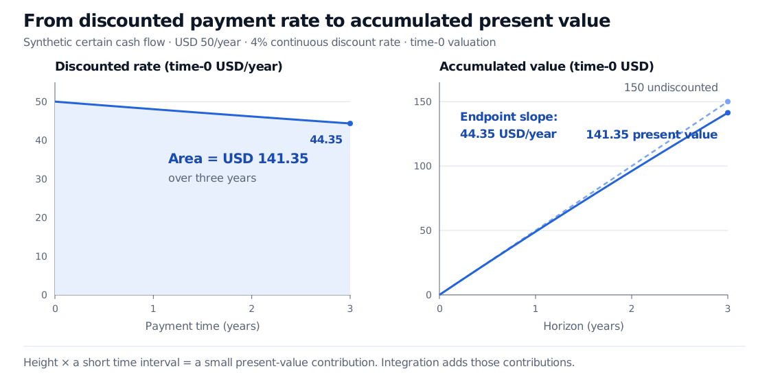
Original synthetic continuous-flow model. The left area and right endpoint represent the same present value; the left panel's height at year 3 equals the right panel's slope there. All values use time-0 USD, with time measured in years.
Now vary the end of the payment horizon, keeping today's valuation date, payment rate and discount rule fixed. The theorem gives
Near the three-year horizon, a small extension years therefore adds approximately dollars of present value. USD 44.35 is a marginal value per extra year, not the exact value of an entire additional year. For a finite extension, use or integrate over the added interval. The slope falls as the horizon grows because later payments receive smaller discount weights; the accumulated value still rises.
At a zero discount rate the integral is simply , giving USD 150 at three years. The expression containing division by the rate must be read through its limit there.
Choosing the next method
Start by identifying the quantity being accumulated and its units. Use an antiderivative when one is convenient: substitution reverses the chain rule, while integration by parts reverses the product rule. Numerical integration handles many cases where an explicit formula is unavailable or the rate is supplied as data.
The economic setup remains separate from the integration method. Payments on discrete dates call for a discounted sum. Uncertain payments require a model of risk and discounting; integration alone supplies neither. Integration against a random driving process belongs to stochastic integration, which has additional definitions and rules.
For a guided development with worked examples, continue to Integration in the Mathematics Primer. The public page previews the lesson; the full lesson requires membership.
Sources
- James Stewart, Single Variable Calculus: Early Transcendentals, 6th ed., Brooks/Cole, 2008, §§5.1–5.4, especially §5.3 on the Fundamental Theorem.
- John C. Hull, Options, Futures, and Other Derivatives, 9th Global Edition, Pearson, 2018, §4.2 on continuous compounding and discounting.
- NIST Digital Library of Mathematical Functions, §1.4(v), equations 1.4.26–1.4.27, for the two Fundamental Theorem identities.