Integration by parts: Definition & Examples

Integration by parts exchanges an integral of one product for a boundary term minus another integral. It is the product rule read backwards. In finance, it can turn a growing cash-flow rate multiplied by a discount factor into an explicit present-value formula. The boundary term is part of the value; losing it can overwhelm the answer.

The identity, including both endpoints

For continuously differentiable functions $u$ and $v$ on a finite interval $[a,b]$ ,

\int_a^b u(t)v'(t)\,dt =\underbrace{u(b)v(b)-u(a)v(a)}_{[uv]_a^b} -\int_a^b v(t)u'(t)\,dt.

The compact notation is

\int_a^b u\,dv=[uv]_a^b-\int_a^b v\,du

. Here

dv

means

v'(t)\,dt

, rather than a second function to differentiate. The fundamental theorem of calculus applied to

(uv)'=u'v+uv'

gives the formula. MIT's introduction derives both forms from this identity.

For an indefinite integral, write

\int u\,dv=uv-\int v\,du

and include one arbitrary constant in the final antiderivative. For a definite integral, evaluate the product at upper minus lower endpoint. There is no arbitrary constant in the resulting number.

Choose $u$ so differentiation simplifies it, and choose $dv$ so an antiderivative is available. A polynomial times an exponential is a useful candidate: differentiating the polynomial reduces its degree, while integrating the exponential preserves its form. This is a strategy, not a promise that every product becomes easier.

A revenue stream that ramps up

Consider a hypothetical contract paying continuously over its first two years. With $t$ measured in years, its cash-flow rate is

c(t)=\alpha t,\qquad \alpha=10\ \text{USD/year}^2,\qquad 0\le t\le T=2\ \text{years}.

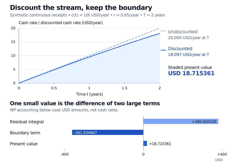
Thus the rate rises from zero to USD 20 per year. The coefficient is USD per year squared because multiplication by time must produce a rate in USD per year. These are continuous receipts:

c(t)\,dt

is an amount of cash. They are not one payment of

c(T)

at maturity.

Assume certain receipts, no fees and a constant continuously compounded discount rate

r=0.05

per year. The discount factor is

e^{-rt}

, with dimensionless exponent

rt

. The time-zero present value is

PV=\int_0^T \alpha t e^{-rt}\,dt.

Use $u=\alpha t$ and $dv=e^{-rt}\,dt$ . Then $du=\alpha\,dt$ and $v=-e^{-rt}/r$ , for $r\ne0$ . Consequently,

\begin{aligned} PV &=\left[-\frac{\alpha t e^{-rt}}{r}\right]_0^T +\frac{\alpha}{r}\int_0^T e^{-rt}\,dt\\ &=-\frac{\alpha T e^{-rT}}{r} +\frac{\alpha}{r^2}(1-e^{-rT})\\ &=\frac{\alpha}{r^2}\left[1-(1+rT)e^{-rT}\right]. \end{aligned}

Both terms have units of USD. Substituting the example's values gives:

Contribution	USD
Boundary term $-\alpha T e^{-rT}/r$	−361.934967
Residual integral $\alpha(1-e^{-rT})/r^2$	+380.650328
Present value	18.715361

The large negative boundary contribution does not mean the contract pays negative cash. It is one term in an algebraic decomposition. The original discounted integrand is nonnegative throughout. Dropping the boundary would give USD 380.65 for receipts whose undiscounted total is only USD 20.

Synthetic continuous cash-flow rate rises from zero to USD 20 per year over two years; its discounted rate ends at USD 18.097 per year. The discounted area is USD 18.715361. Integration by parts decomposes it into a negative USD 361.934967 boundary and a positive USD 380.650328 residual.

Original deterministic example. The top panel shows rates in USD/year; the bottom shows amounts in USD on a common signed scale. The boundary and residual must be combined.

Discounting reduces the value to USD 18.72, versus USD 20 without discounting. This is an illustrative valuation under certain cash flows and a flat discount rate. Uncertain revenue or a non-flat term structure needs its own cash-flow and discounting model.

Check the answer where the formula looks fragile

An antiderivative is

F(t)=-\alpha e^{-rt}\left(\frac{t}{r}+\frac{1}{r^2}\right).

Differentiating it gives $F'(t)=\alpha t e^{-rt}$ : the extra exponential and polynomial terms cancel. Subtracting $F(0)$ from $F(T)$ checks both the minus sign and the lower endpoint.

The formula with $r^2$ in the denominator cannot be evaluated by substituting $r=0$ . The original integral can:

PV\big|_{r=0}=\int_0^T \alpha t\,dt=\frac{\alpha T^2}{2}.

The closed form has the same limit. Its small-rate expansion is

PV=\alpha\left(\frac{T^2}{2}-\frac{rT^3}{3} +\frac{r^2T^4}{8}+\cdots\right).

Near zero, direct subtraction in $1-(1+rT)e^{-rT}$ can lose numerical precision. Use a stable series or numerical integration rather than interpreting that cancellation as a financial discontinuity. In the example the limit is USD 20, and a positive rate makes the first correction negative.

Repeated integration by parts handles higher polynomial cash rates. Writing $I_n=\int_0^T t^n e^{-rt}\,dt$ , for integer $n\ge1$ and $r\ne0$ ,

I_n=-\frac{T^n e^{-rT}}{r}+\frac{n}{r}I_{n-1}, \qquad I_0=\frac{1-e^{-rT}}{r}.

Each step lowers the polynomial degree. Close to zero, this recurrence also needs a stable evaluation method; algebraic correctness alone does not guarantee numerical accuracy.

Ordinary time integration and Itô integration differ

The cash-flow example uses ordinary integration with respect to time. For continuous semimartingales $X$ and $Y$ , the stochastic product formula instead gives

\int_0^T X_t\,dY_t =X_TY_T-X_0Y_0-\int_0^T Y_t\,dX_t-[X,Y]_T,

where

X,Y]_T

is their [quadratic covariation. For Brownian motion starting at zero, this implies

\int_0^T W_t\,dW_t=(W_T^2-T)/2

, rather than

W_T^2/2

. Tehranchi's Cambridge notes give the continuous-semimartingale product formula, p. 54. This correction belongs to Itô integration; it is not an extra term in the smooth cash-flow calculation above.

To practise choosing the factors, repeated integration and cyclic cases, use Examples 1–5 of Integration by Parts. The public page is a preview; the full lesson requires membership.

Sources

James Stewart, Single Variable Calculus: Early Transcendentals, 6th edition (Brooks/Cole, 2008), §7.1 — product-rule derivation, factor choice and repeated integration by parts.
MIT OpenCourseWare, 18.01SC, Introduction to Integration by Parts — indefinite and definite identities.
Michael R. Tehranchi, Stochastic Calculus, Chapter 3, pp. 48 and 54 — quadratic covariation and the stochastic product formula.

The identity, including both endpoints

A revenue stream that ramps up

Check the answer where the formula looks fragile

Ordinary time integration and Itô integration differ

Sources

Related terms

Antiderivative

Continuous compounding

Definite integral

Discount factor

Fundamental theorem of calculus

Itô integral

Present value

Product rule