How volatility models turn return surprises into conditional variance forecasts, and why risk forecasting differs from option-price calibration.
Volatility modelling
Volatility modelling specifies how the scale of uncertain returns behaves, how it can be inferred from available information and how it changes across time or market states. A risk desk might use a model to forecast tomorrow’s return variance; an options desk might use one to value and hedge a collection of contingent payoffs. Those tasks need different targets, data and validation.
A model turns a statement such as “large moves tend to follow large moves” into a rule that can be estimated and tested. It does not turn an uncertain future return into a known outcome.
An estimate or measurement from observations already collected
Forecast risk conditional on recent information
A conditional return variance, often using EWMA, ARCH or GARCH
A forecast of the next distribution’s scale
Explain option prices and hedging exposures
A pricing model consistent with specified option quotes and assumptions
A valuation under a pricing measure; fitting quotes does not establish physical return forecasts
Implied volatility is an option-price input recovered by inversion of a specified pricing formula. A volatility surface organises those quotes across strikes and maturities. Local-volatility and stochastic-volatility models specify dynamics that can be calibrated to such information. A surface alone is not a full account of how future surfaces move.
The distinction between the physical measure P and a risk-neutral measure Q matters: a historical risk forecast cannot simply be substituted for an option-implied input and called a calibrated pricing model. Volatility risk premia, model assumptions and the required horizon can all matter.
A daily variance forecast starts with a return surprise
Let rt be a daily decimal log return and let Ft−1 contain information available before that return. Write
rt=μt+εt,μt=E[rt∣Ft−1],ht=Var(rt∣Ft−1).
Here εt=rt−μt is the innovation, or return surprise. Its conditional mean is zero. A common specification writes εt=htzt with iid standardised innovations zt of mean zero and variance one. This does not require zt to be Gaussian.
The variance ht is available before observing rt; only after that return arrives can its surprise update ht+1. A historical forecast must also use parameter estimates and mean forecasts available at its stated origin.
Removing the conditional mean is part of the model. Squaring the raw return without discussing its mean is an additional assumption, not a general identity. For the synthetic example below, the conditional mean is stipulated to be zero, so the latest return and surprise coincide.
EWMA is an exponentially weighted moving average: the decay factor λ controls how much old variance survives each update. GARCH adds a positive intercept and separates the weights on news and previous variance. Both respond to squared surprises, giving the same next variance for equal positive and negative surprises. An asymmetric model is needed to represent a sign-dependent leverage effect.
Audit the update before trusting the output
Assume a prior daily conditional variance of ht=0.000100, corresponding to a daily standard deviation of 1%. The latest return surprise is +2%=0.02, so its square is 0.000400. Compare two separate, stipulated parameter choices:
EWMA: λ=0.94.
GARCH(1,1): ω=0.000002, α=0.05, β=0.93.
These parameters are not fitted to market data. The EWMA decay factor is also the historical daily choice documented in the 1996 RiskMetrics methodology; it is not a universal optimum.
Contribution, in squared decimal daily-return units
EWMA
GARCH(1,1)
Carried variance
0.94(0.000100)=0.000094
0.93(0.000100)=0.000093
Latest squared surprise
0.06(0.000400)=0.000024
0.05(0.000400)=0.000020
Intercept
None
0.000002
Next daily variance
0.000118
0.000115
Square root: next daily standard deviation
1.0863%
1.0724%
Variance is in squared return units; volatility is its square root. Taking a weighted average of standard deviations instead would produce a different calculation. Neither output says that tomorrow’s return will equal the forecast standard deviation, or that tomorrow’s realised squared return will equal the forecast variance.
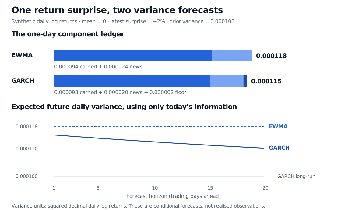
Two component bars produce EWMA variance 0.000118 and GARCH variance 0.000115. Expected future daily variance is flat for the stipulated EWMA recursion and declines toward 0.000100 for GARCH over horizons one to twenty trading days.
Original synthetic calculation. The upper panel decomposes the next-day variance; the lower panel holds today’s information and model parameters fixed. Variance units are squared decimal daily log returns. No future return observations or random paths are plotted.
For the standard GARCH model, ω>0 and α,β≥0 ensure positive variance from a nonnegative starting value. With iid unit-variance innovations, α+β<1 gives a finite unconditional variance,
hˉ=1−α−βω.
Here the sum is 0.98 and hˉ=0.000100. A stationary version of the model can display volatility clustering while having a constant unconditional variance: its conditional variance moves with the information set. The fixed starting state in this example does not assert stationary initialisation. This finite-variance condition is distinct from the more general question of strict stationarity. At the sum-of-coefficients boundary of one, the displayed finite-unconditional-variance formula is unavailable.
For a horizon of k≥1 days, under the stated fixed-parameter GARCH assumptions,
E[ht+k∣Ft]=hˉ+(α+β)k−1(ht+1−hˉ).
The figure therefore shows mean reversion toward hˉ. The corresponding EWMA forecast stays at its latest level if the recursion is interpreted as the conditional second-moment rule with unit-variance standardised innovations. That forecast uses expected future squared surprises, not zero future surprises. EWMA has no separately estimated long-run anchor in this rule; avoid treating it as a covariance-stationary positive-intercept GARCH model. Neither curve is a realised future variance path, and the square root of an expected future variance is generally different from expected future volatility.
A usable model needs more than a recursion
Estimation or calibration chooses parameters for a purpose. A credible forecasting workflow checks the return definition and calendar, models or justifies the conditional mean, records variance initialisation, and checks whether standardised residuals retain serial dependence or dependence in their squares. Heavy tails, asymmetry, changing regimes and bad prices can survive an apparently good variance fit.
Forecast comparison should use later observations, the intended horizon and an appropriate loss or risk criterion. Realised variance proxies are noisy; a better in-sample likelihood alone does not demonstrate better forecasts or valid tail-loss coverage. A conditional variance does not determine the whole loss distribution. Innovation tails and dependence assumptions still matter for value at risk and expected shortfall.
For pricing work, calibration must also respect the chosen quote conventions and inspect arbitrage constraints, parameter stability and hedge behaviour. Reproducing today’s option prices is a different validation task from forecasting tomorrow’s physical returns.
The ARCH and GARCH lesson develops squared-residual testing, Gaussian quasi-likelihood, robust uncertainty estimates and forecast diagnostics. The public page provides a preview; the full lesson requires membership.
Sources
Alexander J. McNeil, Rüdiger Frey and Paul Embrechts, Quantitative Risk Management: Concepts, Techniques and Tools, revised edition, Princeton University Press, 2015, §2.2.2, pp. 55–57 (physical and pricing measures), §4.2.2, pp. 118–119 (GARCH and moment conditions), and §4.2.5, pp. 130–132 (prediction and exponential smoothing).