Read implied volatility across strike and expiry, distinguish annualised volatility from total variance, and see why interpolation needs price-based arbitrage checks.
Volatility surface
A volatility surface is the map of implied volatilities across option strikes and times to expiry for one underlying, observed at one valuation time. Each height is the volatility that makes a specified pricing formula reproduce that option's price. A horizontal cut at one expiry gives a volatility smile or skew; a cut through a chosen strike or moneyness coordinate gives a volatility term structure.
The surface answers a practical question: which volatility belongs to this particular contract? A dealer pricing a short-dated out-of-the-money call cannot simply borrow the one-year at-the-money volatility. Both its strike position and its horizon differ. Hull's §20.5 introduces the surface as the combination of strike slices and the term structure, including the need to interpolate between quoted contracts.
Here T is remaining time in years, r and q are the chosen continuously compounded financing rate and proportional dividend yield, and C is a premium per underlying unit. Those conventions are part of the definition. An American premium put into a European inversion does not produce a directly comparable surface.
Absolute strike K is only one possible horizontal coordinate. Another is moneyness relative to the matching forward price:
k=log(F0,TK),F0,T=S0e(r−q)T.
The forward formula here assumes constant deterministic rates and proportional yield. More general carry needs the appropriate forward curve. At-the-money-forward means K=F0,T, or k=0; it need not mean K=S0. A fixed-k term structure can therefore follow different absolute strikes at different expiries.
Three labels prevent common misreadings:
Surface feature
Hold fixed
Read
Smile or skew slice
Expiry T
How IV changes across strikes or moneyness
ATM-forward term structure
k=0
How ATM-forward IV changes with expiry
Fixed-strike term structure
Absolute strike K
How the IV of that strike changes with expiry
Some markets quote delta rather than strike, while FX quotes also specify ATM, risk-reversal and butterfly conventions. Delta itself has spot/forward and premium-adjustment variants. A “25-delta” coordinate is incomplete without its convention; Reiswich and Wystup explain the FX delta variants. Normal (Bachelier) volatility and lognormal Black volatility also have different units; the Eris Options Analytics Guide distinguishes price- and rate-based volatility measures. Convert quotes to a common contract and pricing convention before comparing their heights.
An original nine-contract surface
Consider a synthetic zero-carry example with spot and every forward equal to USD 100, European calls, no dividends and r=q=0. Construct prices as the equally weighted mixture
This averages prices, then inverts each result to one BSM implied volatility. It does not average the two volatilities. The construction is a probability mixture of two valid zero-carry lognormal martingale price families, which gives a coherent family of European prices across strikes and expiries.
Time to expiry
Strike USD 80: call / IV
Strike USD 100: call / IV
Strike USD 120: call / IV
0.25 years
20.5930 / 32.91%
4.9800 / 24.98%
1.0737 / 31.69%
1 year
23.2155 / 28.80%
9.9199 / 24.93%
4.6677 / 27.82%
2 years
25.9217 / 27.17%
13.9537 / 24.86%
8.2208 / 26.50%
Prices are USD per underlying unit; IVs are annualised. Each cell is a separate valuation today, rather than a prediction of where a currently traded contract's quote will move.
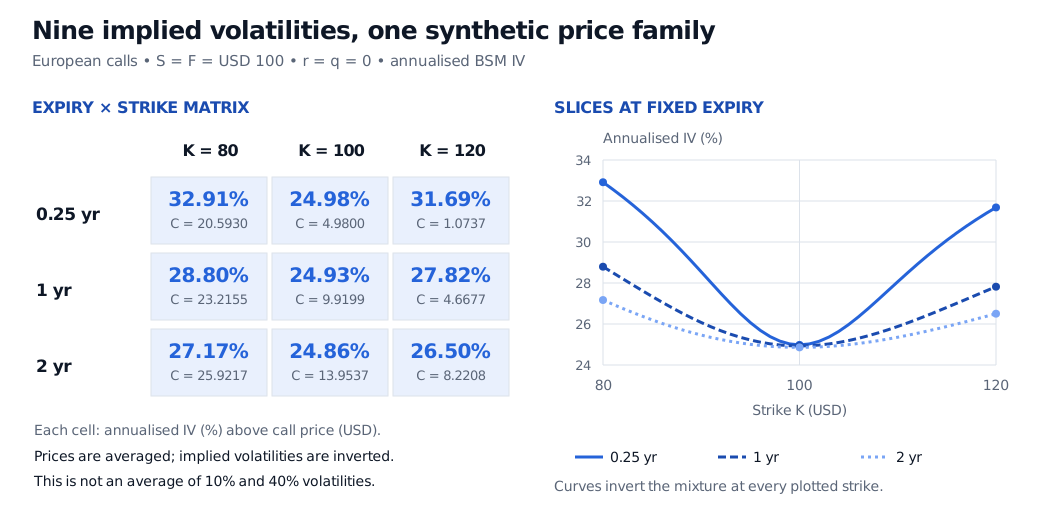
A nine-cell synthetic surface at strikes USD 80, 100 and 120 and expiries 0.25, 1 and 2 years. IV rows are 32.91%, 24.98%, 31.69%; 28.80%, 24.93%, 27.82%; and 27.17%, 24.86%, 26.50%. Three inverted strike slices show wings flattening with expiry.
Original synthetic European call example. Each cell shows IV above its USD call price; curves invert the same mixture at every plotted strike. Zero carry makes spot and forward equal at all expiries.
Suppose a desk needs the three-month USD 120 call. The relevant surface height is 31.69%, giving a premium of USD 1.0737. The two-year contract at that strike instead uses 26.50% and costs USD 8.2208. A lower annualised IV can accompany a higher premium when the maturity changes; vega compares price sensitivity to volatility while holding the contract's other inputs fixed.
The term-structure trap: volatility is an annual rate
Surface work often uses total implied variance:
w(k,T)=σimp(k,T)2T.
Use decimal volatility: 25% is 0.25, not 25. Annualised variance has units of inverse years, so multiplying by T in years gives dimensionless total variance. It is a pricing coordinate; it is not automatically an expectation of future realised variance.
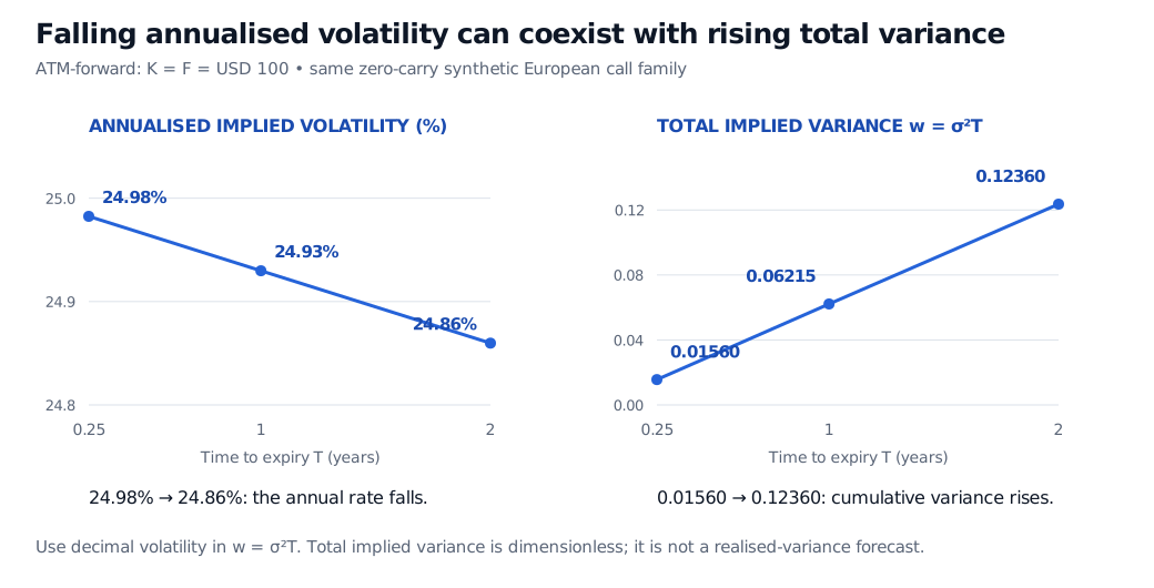
In the example, ATM-forward IV declines slightly with maturity, while total implied variance rises:
T in years
ATM-forward IV
w(0,T)
0.25
24.98%
0.01560
1
24.93%
0.06215
2
24.86%
0.12360
Separate ATM panels show annualised IV falling from 24.98% to 24.93% to 24.86%, while dimensionless total implied variance rises from 0.01560 to 0.06215 to 0.12360 at 0.25, 1 and 2 years.
Same synthetic family, two different quantities and separate vertical scales. The annualised volatility need not increase for cumulative implied variance to increase.
For the zero-rate, zero-dividend European example, calls at a fixed strike cannot become cheaper with maturity: conditional Jensen's inequality applied to a martingale stock and its convex call payoff gives that ordering. The mixture preserves it.
With deterministic proportional carry, a useful generalisation works at fixed log-forward-moneyness. Set D(0,T) to the discount factor and normalise the call as c=C/[D(0,T)F0,T]. Under the standard martingale and exercise assumptions, this normalised price is nondecreasing with maturity at fixed k; because the normalised Black price increases with w, so must w(k,T). Gatheral and Jacquier's Lemma 2.1 states the calendar condition with its proportional-dividend assumption.
This is not a rule that raw IV must rise, nor an unconditional rule about unadjusted fixed-strike prices across all markets. Fixed cash dividends, exercise rights, discounting and carry can change the comparison. Nor is a difference of two vanilla total implied variances generally the price or IV of a forward-starting option: that payoff depends on joint dynamics between the dates.
A smooth picture still needs price checks
Observed quotes occupy a sparse grid. Interpolation fills gaps; extrapolation supplies wings beyond liquid quotes. A visually smooth IV plot can still imply impossible prices. The useful audit starts by converting the surface back to calls on a consistent basis:
Bounds and vertical spreads: at a fixed expiry, calls respect their model-consistent lower and upper bounds and decrease with strike; their slope cannot be more negative than the discounted unit payoff allows.
Butterflies: call prices are convex in strike. For equally spaced strikes, C(K−h)−2C(K)+C(K+h)≥0; otherwise a nonnegative butterfly payoff has a negative purchase price.
Calendars: compare the properly normalised contracts under the relevant carry and exercise assumptions, including the fixed-k total-variance test where applicable.
These are checks on prices and contracts, not on whether the IV mesh looks tidy. In the synthetic example, the mixture preserves strike monotonicity, convexity and the zero-carry calendar ordering because each component has those properties. Passing a finite grid of tests, however, does not prove that an arbitrary interpolator is safe between nodes or in its extrapolated tails. Gatheral and Jacquier develop constrained SVI fitting and interpolation specifically to preserve static consistency.
Actual quote work also needs timestamps, reliable bid and ask ranges, dividend and forward inputs, day counts and settlement terms. A midpoint violation can disappear inside executable spreads. Far-wing, low-vega quotes may have a wide IV uncertainty range even when their premium range looks small. Fitting every noisy midpoint exactly can worsen the surface.
The existing public Volatility Surface explorer helps inspect how ATM level, skew, curvature and term slope alter a shape. It uses a synthetic parametric formula, with a constant forward across expiries; it is not live data, a calibration, or a guarantee of arbitrage-free prices. Its formula is also different from the mixture used in this article.
A surface is today's cross-section, not tomorrow's dynamics
The surface labels contracts by (K,T). Local volatility instead supplies an instantaneous diffusion coefficient σloc(S,t) indexed by future asset state and time. The two functions are related through a model and calibration; they are not interchangeable inputs.
A complete, sufficiently regular European surface can identify risk-neutral terminal marginals under suitable assumptions. It does not uniquely specify how the stock and volatility evolve jointly through time. Models agreeing on today's vanilla prices can disagree on barriers, forward starts and future smile behaviour. It is also distinct from historical volatility: risk-neutral option prices embed pricing and risk preferences, so a high wing IV is not directly a physical probability forecast.
For a curriculum bridge, §4.2 of Volatility Smiles as the Bridge Out introduces surface inversion; full lesson access requires membership, with a public preview. Use the calendar conditions stated above when comparing expiries.
Practice
1. Does falling IV fail the calendar test? European calls have zero rates and dividends. At the same ATM-forward strike, six-month IV is 30% and one-year IV is 24%. Do these two quotes violate the nondecreasing-total-variance condition?
Answer. No. With T in years and decimal IV, w1=0.302×0.5=0.045, while w2=0.242×1=0.0576. Total implied variance increases even though annualised IV falls. This passes this one comparison; it does not establish that every strike slice or interpolated point is consistent.
2. Find the price defect. Matched European calls at strikes USD 90, 100 and 110 cost USD 16, 12 and 6 per unit. Ignore costs and spreads, and set rates to zero. Are decreasing call prices enough to make this slice safe?
Answer. No. Buy the 90 call and 110 call and sell two 100 calls. Its purchase price is 16−2(12)+6=−2: it pays you USD 2 initially. At expiry its payoff is max(10−∣ST−100∣,0), which is never negative. The defect is lack of convexity, despite all three call prices decreasing with strike. Under the stipulated executable, frictionless assumptions this gives a static arbitrage.
Sources
John C. Hull, Options, Futures, and Other Derivatives, 9th Global Edition, §§20.4–20.5: alternative strike coordinates, ATM conventions, volatility term structures and surface interpolation; §20.7: the pricing model's role. The example, prices and figures here are original.
Jim Gatheral, The Volatility Surface: A Practitioner's Guide (Wiley, 2006), Chapter 1, “A Brief Review of Dupire's Work” and “Local Volatility in Terms of Implied Volatility”: implied versus local volatility, total implied variance and log-forward coordinates.