A volatility smile plots implied volatility across strikes for one expiry. Build a consistent synthetic smile, measure flat-volatility pricing errors, and distinguish a smile from skew and a forecast.
Volatility smile
A volatility smile is the pattern of implied volatility across option strikes for one underlying and one expiry, observed at the same valuation time. In the familiar U-shaped version, options away from the at-the-money region have higher implied volatilities than those near it. Traders also use “smile” more broadly for a non-flat strike slice, including an asymmetric volatility skew.
The useful question is: how much volatility must the chosen pricing formula use to reproduce each option price? A smile reveals that one constant volatility cannot reproduce the entire cross-section. It helps a trader compare relative option prices and shows a risk manager where using only an at-the-money volatility loses information.
Prices first, implied volatilities second
Fix a European call’s underlying price S, strike K, remaining life T in years, continuously compounded financing rate r and continuous dividend yield q. Its Black–Scholes–Merton implied volatility solves
CBSM(S,K,T,r,q,σimp(K,T))=Cquote(K,T).
Here Cquote can be an observed premium or an explicitly hypothetical price. With positive expiry, the BSM call price increases strictly with volatility; an interior price between the model’s zero-volatility lower limit and upper limit therefore has one finite positive IV. Prices at or outside those boundaries require separate treatment.
A smile is a price coordinate under stated conventions. Changing the dividend assumption, forward, expiry calculation or pricing model can change the inferred IV even when the premium stays fixed. An American option requires an exercise-aware treatment; a European BSM inversion does not automatically account for its early-exercise value.
Use moneyness to put strikes on a comparable scale. For a known forward F to the option’s expiry, useful horizontal coordinates are
FKork=log(FK).
Forward-at-the-money means K=F, or k=0. It need not mean K=S. Under the simple deterministic continuous-carry convention, F=Se(r−q)T. Always say which coordinate and ATM convention a chart uses.
One expiry, five prices
Imagine checking a one-year European option sheet on an underlying at USD 100, with zero interest and no dividends, so its forward is also USD 100. The following prices are an original synthetic illustration, constructed before any IVs are calculated.
For every strike, average two complete BSM call-price families: one with 10% volatility and one with 40%, each with weight one half:
This can be viewed as a risk-neutral model that selects one of two martingale price processes. Both have the same initial price and forward. The 50/50 weights are modelling weights under the pricing measure, not a forecast that the real world has two equally likely volatility regimes.
Strike K (USD)
Forward moneyness K/F
Call price (USD per underlying unit)
Annualised BSM IV
80
0.80
23.2155
28.80%
90
0.90
15.6418
26.07%
100
1.00
9.9199
24.93%
110
1.10
6.5310
25.88%
120
1.20
4.6677
27.82%
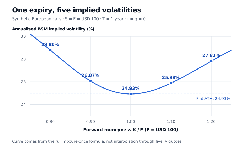
Each IV comes from a separate inversion of that row’s unrounded price. There is one underlying model behind the sheet, yet the implied volatilities vary by strike. None equals an assertion that the underlying “really has” a separate constant volatility for each option.
Synthetic one-year smile: IV falls from 28.80% at strike 80 to 24.93% at 100, then rises to 27.82% at 120.
Original synthetic mixture; S=F=100, T=1 year, r=q=0. Both component price families use the same terms. The curve is generated by the full mixture formula, not an arbitrary curve through five points.
The construction matters. Each component’s call prices decrease and are convex in strike, and a positive weighted average preserves those properties and the price bounds. This establishes consistency across the full strike family. Checking five prices alone would not prove that an arbitrary interpolation or extrapolation is free of arbitrage.
What a flat ATM volatility misses
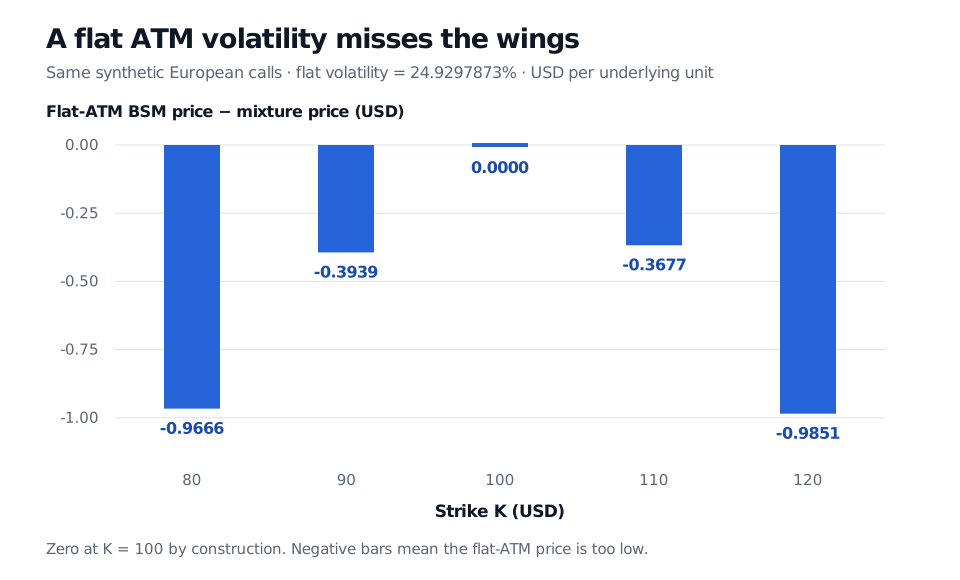
Suppose the sheet is replaced with its ATM IV, 24.9297873%, at every strike. The 100-strike call still costs USD 9.9199. The 80-strike call instead costs USD 22.2489, versus USD 23.2155 on the synthetic sheet: an underpricing of USD 0.9666 per underlying unit.
Using flat ATM volatility produces call pricing errors of minus 0.9666, minus 0.3939, zero, minus 0.3677 and minus 0.9851 USD at strikes 80 through 120.
Original pricing comparison for the same synthetic European calls. Error is flat-ATM BSM price minus mixture price. Negative means underpriced relative to this sheet; it is not a trading profit.
The 80-strike call is in the money, but its matching 80-strike put is out of the money. With zero carry, put–call parity gives P=C−S+K: the mixture put costs USD 3.2155, while flat ATM volatility gives USD 2.2489. The same dollar error appears in both contracts. Matching European calls and puts have the same IV when their prices satisfy parity and the inversion uses consistent forwards, discounting and other terms. Mismatched exercise styles, stale quotes or inconsistent inputs can spoil that comparison.
A smile does not have to be symmetric
A U-shaped smile has two elevated wings; it need not be symmetric in strike or have its minimum exactly at ATM. A downward skew instead has higher IV at low strikes than at high strikes. The conventional equity-index downside skew is an example: a low-strike out-of-the-money put can have higher IV than a high-strike out-of-the-money call. That comparison uses different strikes, so it does not contradict matched-strike call–put parity. Hull’s equity and currency examples and CME’s explanation of smile curvature distinguish these shapes.
Higher low-strike IV describes relatively expensive downside option payoffs under the chosen quote convention. It can reflect the pricing of tail risk, protection demand and risk premia. It does not, by itself, identify the physical probability of a crash. Nor is an IV reading the same object as realised volatility, which is calculated from observed returns. Inferring a pricing-measure distribution from a sufficiently complete, consistent option-price curve is a different exercise from forecasting real-world outcomes.
To explore shapes, open the Volatility surface explorer and compare Smile, Downside skew and Flat. Change curvature and skew to see how they differ. Its presets are synthetic parametric shapes: they do not reproduce this article’s mixture prices, use live quotes or guarantee arbitrage-free prices. The quotation discussion in Volatility Smiles as the Bridge Out offers a further introduction; the link is a public preview and the full lesson requires membership.
Reading a smile without overreading it
Compare like with like: same underlying, expiry, valuation time, exercise and settlement terms, with a coherent forward and discount curve. Record whether a point comes from bid, ask, midpoint or a model. A wide bid–ask spread can produce a wide IV range, especially when vega is low. A jagged wing may reflect sparse or stale quotes rather than a precisely identified tail shape.
A higher-IV option is not automatically an attractive sale. The quote can pay for risks that a flat-volatility model omits, and comparing two IVs does not remove differences in payoff exposure. The underpricing in the figure is a comparison against our stipulated synthetic sheet; it is not an executable arbitrage claim.
Finally, a smile fixes one expiry. Stacking slices across expiries produces a volatility surface. Even a model that fits today’s vanilla prices can imply different future smile movements from another model with the same fit. That matters for hedging and path-dependent options; a static fit alone does not settle the dynamics.
Practice
1. Smile or skew? At one valuation time and one expiry, three hypothetical European-option quotes imply 27%, 23% and 21% volatility at strikes 90, 100 and 110. Which description fits the displayed region: a U-shaped smile, a downward skew, or flat volatility? What is the low-to-high-strike IV difference?
Answer. A downward skew: IV decreases as strike increases. The difference is 27%−21%=6 volatility percentage points. There is no rising right wing in these three quotes, so they do not display a U-shape. They also do not say there is a 27% probability of a downside move. No claim about a fully calibrated or arbitrage-free price curve follows from these three illustrative IVs alone.
2. Must the put have a different IV? A hypothetical European call costs USD 6.25 per underlying unit, with S=120, K=130, T=0.5 years and r=q=0. A matched put satisfies parity. Find its price. If BSM inversion gives the call IV 29.85% to two decimals, should a consistent put inversion produce a different IV because the put is in the money?
Answer. Parity gives P=6.25−120+130=16.25 USD per underlying unit. The put has the same IV: approximately 29.85% annualised, with a more precise value of approximately 29.8518211%. The BSM formula itself satisfies parity at every volatility; the volatility fitting the call therefore fits the parity-consistent put. Being in or out of the money changes the payoff, not this matched-contract identity.
Sources
John C. Hull, Options, Futures, and Other Derivatives, 9th Global Edition, Chapter 20, especially §§20.1–20.4: matched European call/put smiles, currency smiles, equity skew and alternative moneyness coordinates. Local source text checked; numerical examples here are original.
Jim Gatheral, The Volatility Surface: A Practitioner’s Guide, Wiley, 2006, Chapter 1, pp. 1–2: different implied volatilities can arise from consistent common dynamics; fitting and hedging are distinct tasks.