Historical volatility measures past return dispersion. Calculate a five-day log-return estimate and distinguish sample conventions, annual scaling and future risk.
Historical volatility
Historical volatility measures the dispersion of an asset’s past returns over a specified window, commonly using their standard deviation. A risk system might use it to size positions or compare recent turbulence with a longer baseline. The number describes the chosen history; treating it as tomorrow’s risk estimate adds a forecasting assumption.
“Historical” does not identify a unique calculation. A reproducible quote must state the return definition, observation frequency, lookback window, estimator and annualisation convention.
Start with returns, not price levels
For positive prices P0,…,Pn observed at equal intervals, with no intervening distributions, define log returns by
ri=log(Pi−1Pi),i=1,…,n.
There are n+1 price observations but only n returns. A standard sample calculation is
rˉ=n1i=1∑nri,s2=n−11i=1∑n(ri−rˉ)2,s=s2.
Here s2 is return variance, and s is volatility at the observation frequency. Daily returns produce a daily standard deviation. Taking the standard deviation of price levels instead would produce a quantity in price units, sensitive to the nominal share price.
The divisor n−1 accounts for estimating the mean from the same sample. Under independent, identically distributed returns with finite variance, it makes s2 unbiased for that variance; it does not make s unbiased for the standard deviation. Basic Statistics and Regression develops this sample-statistic framework. The full lesson is available with a signed-in free account.
Five daily moves, fully specified
Take these five synthetic one-trading-day log returns, entered as decimals:
−0.02,−0.01,0,0.01,0.02.
These correspond to log returns of −2%, −1%, 0%, 1% and 2%; they are not simple percentage price changes. Stipulate equal daily intervals, no dividends or other distributions, and no missing observations. This small window teaches the arithmetic rather than proposing an adequate risk-estimation sample.
The mean is zero and the sum of squared deviations is 0.001. Consequently,
s2=5−10.001=0.00025,s=0.00025≈0.0158114.
The daily historical volatility is 1.5811%. Dividing the squared deviations by n=5 instead gives descriptive variance 0.0002, and standard deviation 1.4142%. Both conventions occur in statistical work; they must be named rather than silently interchanged. A zero-mean model or a particular likelihood estimator also needs its own declared convention.
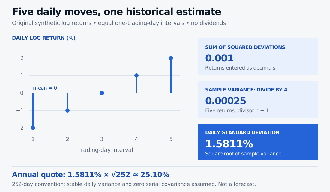
Five synthetic daily log returns of minus 2%, minus 1%, zero, 1% and 2% have mean zero, squared-deviation sum 0.001, sample variance 0.00025 and daily standard deviation 1.5811%. Annual scaling by square root of 252 gives approximately 25.10%.
Original synthetic equal-day log returns. The sample estimator uses divisor four. The annual quote assumes a 252-trading-day year, stable daily variance and zero serial covariance; it is not a forecast.
The annual quote adds a time convention
For a stipulated year of A equal trading-day intervals, the usual annualised volatility quote is
σ^annual=sA.
With A=252, the example gives 252×0.00025≈0.250998, or 25.10% annually. The observed window remains five days; annualising it does not create a year of observations.
The scaling reflects variance addition for summed log returns with equal finite variance and zero serial covariance. Nonzero serial covariances contribute extra terms. Volatility clustering also warns that a stable unconditional average need not describe the next period’s conditional risk, even when returns themselves are uncorrelated. A square-root quote alone supplies neither a forecast nor a probability bound on losses.
What changes the estimate
Window and weighting. A short rolling window reacts quickly but is sensitive to individual observations. A longer window mixes more market conditions. An old large move leaving the window can lower the estimate without any new calm-market evidence. Equal weighting, exponential weighting and a conditional volatility model are different estimators.
Return basis and data cleaning. Declare log versus simple returns, price versus total returns, closing-time conventions and missing-data treatment. Adjust splits and other corporate actions consistently. A vendor’s “adjusted close” label does not establish its dividend policy. Equities, Indices and Corporate Actions explains how these events enter historical return data; its public preview is available and the full lesson requires membership.
Comparison target.Implied volatility is inferred from option prices through a pricing model. It concerns a specified option horizon and embeds pricing effects absent from a backward-looking standard deviation. Matching annual units is insufficient to make the two interchangeable.
The term overlaps with realised volatility, but that label can refer to a different sampling frequency, a sum of squared returns or a contract-specific formula. Compare the definitions and dates before comparing the numbers.
Sources
John C. Hull, Options, Futures, and Other Derivatives, 9th edition, Global Edition (Pearson, 2018), Chapter 15 §15.4, pp. 348–349: historical log-return estimation, the sample divisor, time scaling and dividend treatment. The example here is original and synthetic.