Annualised volatility: Definition & Examples

Annualised volatility is the standard deviation of returns expressed on a one-year scale. It lets a risk report put daily and monthly estimates on a common clock. The conversion usually multiplies the observed period's volatility by the square root of the number of periods per year. Whether that number also describes the dispersion of an actual year's return depends on the return definition and the assumptions behind the conversion.

A label such as “15.875% annualised” therefore needs context: what returns, sampled when, estimated over which window, using which year convention? Annualising a short sample does not create a year's worth of observations or establish a reliable forecast.

Why 1% becomes 15.875%

Take a synthetic model of daily log returns with daily standard deviation

\sigma_d=0.01

, stable finite daily variance and zero serial covariances. Declare 252 equal observation periods per model year. Then

\sigma_{\mathrm{ann}}=\sqrt{252}\,\sigma_d =\sqrt{252}\times0.01 \approx0.1587451=15.875\%.

The underlying variance scales from

0.0001

252\times0.0001=0.0252

, in squared decimal-return units. Standard deviation is its square root. Multiplying 1% by 252 would give 252%; that uses the wrong scaling for dispersion.

Why the square root? For any finite-variance returns $r_1,\ldots,r_q$ ,

\text{Var}\!\left(\sum_{t=1}^{q}r_t\right) =\sum_{t=1}^{q}\text{Var}(r_t) +2\sum_{i<j}\text{Cov}(r_i,r_j).

Common period variance

\sigma_d^2

and zero serial covariances reduce this to

q\sigma_d^2

. Taking the square root gives

\sqrt q\,\sigma_d

. Independent, identically distributed returns with finite variance are sufficient; normality is unnecessary, and independence is stronger than this variance calculation needs.

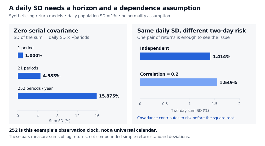
With daily log-return SD of 1%, zero serial covariances give sum SD of 1%, 4.583% and 15.875% over 1, 21 and 252 periods. With the same daily SD, two-day sum SD is 1.414% under independence and 1.549% with correlation 0.2.

Original synthetic log-return models. Left: a fixed 252-period year and zero serial covariances. Right: two different two-day joint distributions with the same daily population standard deviation. All bars show standard deviations of return sums.

Add the right kind of return

For positive, total-return-adjusted index levels $V_t$ , define the log return as $r_t=\log(V_t/V_{t-1})$ . It adds exactly across time:

\sum_{t=1}^{q}r_t=\log(V_q/V_0).

The square-root calculation above therefore gives the standard deviation of the year's log return, under its stated model. If prices are used instead of a total-return index, account for dividends and other distributions consistently with the intended return measure.

Simple returns,

R_t=V_t/V_{t-1}-1

, compound:

R_{1:q}=\prod_{t=1}^{q}(1+R_t)-1.

Multiplying their daily standard deviation by

\sqrt{252}

is a common annual-scale quotation, but the variance-of-a-sum identity applies to

\sum R_t

, not to that product. It does not generally give the exact standard deviation of the compounded annual simple return. Small daily returns can make the approximation useful; they do not make the two random variables identical.

The Financial Return Characteristics lesson develops this distinction and explains how dependent return magnitudes can coexist with uncorrelated signed returns. The public page is a preview; the complete lesson requires membership.

Two days reveal the dependence problem

Keep daily log returns at either −1% or +1%, each with probability one half. Each day's population variance is

0.0001

. If the days are independent, their sum is −2%, zero or +2%, with probabilities

0.25

0.50

and

0.25

. Its variance is

0.0002

and its standard deviation is 1.414%.

Now change only their joint probabilities:

First day	Second day	Joint probability
−1%	−1%	0.30
−1%	+1%	0.20
+1%	−1%	0.20
+1%	+1%	0.30

Both daily marginal distributions are unchanged, but the days now have correlation $0.2$ and covariance $0.00002$ . Hence

\text{Var}(r_1+r_2) =0.0001+0.0001+2(0.00002) =0.00024,

so the two-day standard deviation is 1.549%. The daily figure alone could not reveal this difference. A single two-day correlation also cannot determine annual risk: longer horizons require the relevant covariance terms at all lags.

For a covariance-stationary return process, let $\gamma_k=\text{Cov}(r_t,r_{t-k})$ . The general expression is

\text{Var}\!\left(\sum_{t=1}^{q}r_t\right) =q\gamma_0+2\sum_{k=1}^{q-1}(q-k)\gamma_k.

Positive weighted serial covariance increases sum variance; negative weighted serial covariance reduces it. Lo's time-aggregation analysis develops this correction and explicitly distinguishes its sum approximation from compounded simple returns.

Volatility clustering is a separate issue. Dependence in squared returns does not by itself establish nonzero covariance of signed returns. Even with uncorrelated returns, a forecast made today may need different conditional variances for successive future periods. Annualising today's conditional daily volatility does not establish that every future day will have that variance.

A scale conversion, an estimate, or a forecast?

A model standard deviation $\sigma_d$ is a population quantity. A historical estimate $s_d$ is computed from data. One centred sample convention, for $n\ge2$ , is

s_d^2=\frac{1}{n-1}\sum_{t=1}^{n}(r_t-\bar r)^2, \qquad \widehat\sigma_{\mathrm{ann}}=\sqrt q\,s_d.

Here $n$ counts observations in the estimation window; $q$ counts observation periods per declared year. Changing the lookback changes

s_d

, not automatically

q

. Other historical or realised estimators may use different centering, divisors or weights; annualisation does not reconcile those choices.

A 252-period convention is used in NYU V-Lab's published volatility scale. It is not a universal law about daily data. A crypto series sampled at every 24-hour interval might instead use a declared 365-period convention. Switching the multiplier while leaving the observation clock unexplained makes comparisons ambiguous. Monthly, trading-day and calendar-day inputs require matching conventions.

Finally, annualised volatility is a dispersion measure, not an expected return, a maximum loss or a probability guarantee. To compare two figures, align the return basis, sampling clock, estimation method, window and treatment of serial dependence. To use one as a forecast, also justify why its estimated variance and dependence structure remain relevant to the future horizon.

Sources

John C. Hull, Options, Futures, and Other Derivatives, 9th Global Edition (Pearson, 2018), §15.4, pp. 347–350: log-return volatility, historical sample estimation and trading-time annualisation.
NYU Stern V-Lab, Volatility Welcome Page Help, “Annualized Numbers”: its daily-to-annual quotation convention.
Andrew W. Lo, “The Statistics of Sharpe Ratios”, Financial Analysts Journal 58(4), 2002, pp. 40–41, “Time Aggregation”: covariance contributions and the explicit treatment of compounded simple returns as a separate issue.

Why 1% becomes 15.875%

Add the right kind of return

Two days reveal the dependence problem

A scale conversion, an estimate, or a forecast?

Sources

Related terms

Covariance

Return

Variance

Volatility

Volatility clustering