A return measures an investment's gain or loss relative to the capital used to earn it, over a stated period. It puts investments of different sizes on a comparable scale. For a quant, the choice of return also determines how a backtest compounds and which observations belong in a risk estimate.
For positive starting wealth and ending wealth , with no external deposits or withdrawals, the simple return is
Wealth must include the investment income being measured. State the currency, holding period and treatment of costs: a price change alone, a total return including distributions, and a return after fees describe different things.
The percentage changes its own base
Consider a synthetic, fully funded holding worth USD 100 → USD 110 → USD 99 over two equal-length periods. There are no distributions, external flows, transaction costs, fees, taxes or financing charges.
| Interval | Starting wealth | Ending wealth | Simple return | Gain or loss |
|---|---|---|---|---|
| First period | USD 100 | USD 110 | +10% | +USD 10 |
| Second period | USD 110 | USD 99 | −10% | −USD 11 |
| Both periods together | USD 100 | USD 99 | −1% | −USD 1 |
The second loss is 10% of 110, while the first gain was 10% of 100. Adding the two percentages erases that change of base. Link their gross growth factors instead:
Thus the cumulative simple return is , or −1%. A gross growth factor of 0.99 means that each initial dollar has become 99 cents; it does not mean a positive 99% return.
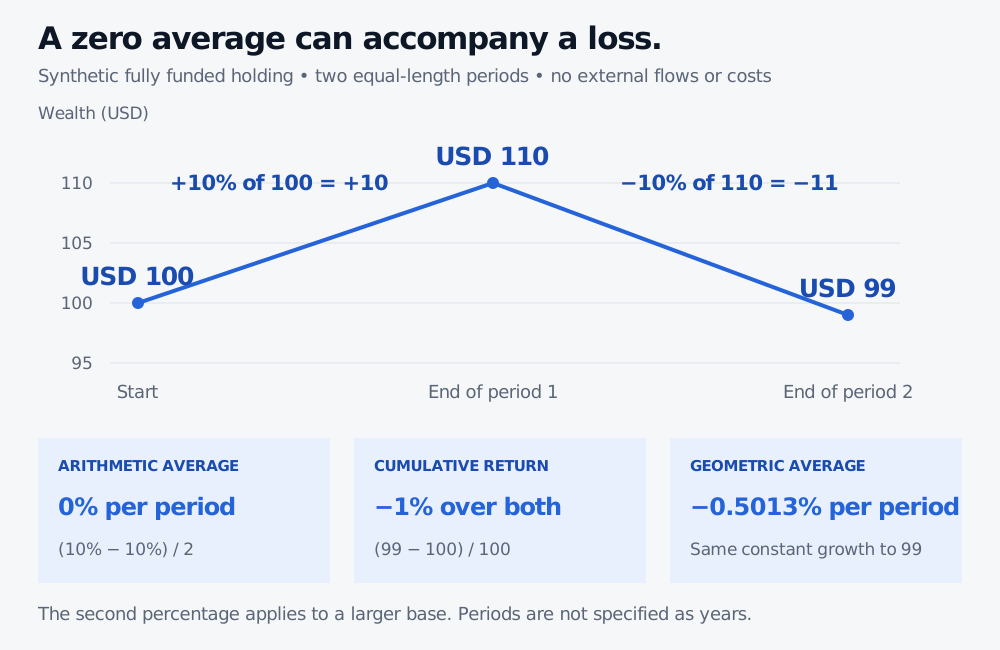
Original synthetic wealth path over two equal-length periods. The gain is USD 10 and the loss is USD 11. No flows, distributions or costs; the periods are not specified as years.
An average answers a different question
The arithmetic average of the two period returns is . That correctly describes their sample average. It does not describe the change in invested wealth, and two observations do not establish an expected future return.
The geometric average asks which constant simple return, applied in each period, would reproduce the ending wealth:
Compounding this unrounded rate twice gives the same −1% cumulative return. Neither average is an annual return here: the example supplies two comparable periods, without specifying their calendar length. Annualisation needs a stated horizon and convention.
Logs add; simple returns compound
For strictly positive wealth, a log return uses the natural logarithm:
On this path, the log returns are approximately 0.09531018 and −0.10536052, in decimal log units. Their exact sum is . Convert back to a cumulative simple return with . Adding logs preserves the compounding identity; it does not turn the log sum into the simple percentage return. These definitions and conversions are developed in Eric Zivot's Return Calculations, §§1.2.2–1.2.3.
A fully funded, limited-liability holding can lose 100% of its value. Its simple return is then −1, but a finite log return no longer exists because ending wealth is zero. A return calculated on a leveraged account needs its own equity and financing conventions.
Count income once, and separate it from deposits
For one share bought at price , ending at , with a cash dividend paid at the end of the period, the simple total return before costs and taxes is
This convention holds the share throughout and treats the final cash payment separately from its price. Earlier distributions require an explicit cash-holding or reinvestment assumption. If the input is already a total-return series including reinvested dividends, adding dividends again double-counts income. S&P Dow Jones Indices distinguishes price indices from total-return indices that include reinvested dividend income.
An investor's deposit is different: it increases account wealth without being an investment gain. When money enters or leaves during a measurement interval, raw balance changes need a flow-aware performance calculation. Likewise, deduct transaction costs only if they have not already been included in the series.
For the next step from return calculation to statistical modelling, Financial Return Characteristics explains simple and log returns, portfolio aggregation, heavy tails and volatility clustering. The public page is a preview; the full lesson requires membership.
Sources
- Elton, Gruber, Brown and Goetzmann, Modern Portfolio Theory and Investment Analysis, ninth edition, Wiley, ©2014, Chapter 2, p. 19: holding-period return and the treatment of income received within the period.
- Eric Zivot, Introduction to Computational Finance and Financial Econometrics with R: Return Calculations, §§1.2.2–1.2.3: simple returns, compounding, geometric averages and logarithmic returns.
- S&P Dow Jones Indices, Index Mathematics Methodology: price and total-return index construction.