Forecast future return variance with an auditable EWMA update, distinguish realised and implied quantities, and align information, horizon, square roots and evaluation.
Volatility forecasting
Volatility forecasting estimates the dispersion of future returns using information available at a stated forecast time. A common target is the next period’s conditional variance; its square root is the corresponding conditional volatility. A risk manager can use that forecast to adjust exposure before the next session, but it says neither which direction the asset will move nor how large tomorrow’s realised return must be.
The target needs a contract: which asset and return definition, which future interval, which information cutoff, and which units? A forecast for tomorrow’s close-to-close log return includes overnight risk. A forecast for tomorrow’s open-to-close return covers a different exposure, even if both are labelled “daily”.
Three quantities that can share a volatility label
Quantity
What it answers
What must match in a comparison
Conditional forecast
How much dispersion does a model assign to a future return, given today’s information?
Forecast origin, return definition and future horizon
Which volatility input makes an option-pricing model reproduce a quote?
Option terms, pricing model, timestamp and expiry
Option-implied quantities contain forward-looking information, but they are extracted from prices of risky claims. They are not automatically unbiased forecasts of physical return variance. Nor is a historical standard deviation automatically a conditional forecast: using it to predict the future adds a stability assumption. OIC describes the historical-versus-option-implied measurement distinction.
Let Ft represent the information available after day t, and let Rt+1 be the next daily decimal log return. The variance target is
That definition is separate from the method used to estimate it. Different forecasting models can assign different variances to the same future return.
One large return, one auditable update
Imagine an equity-risk desk using a synthetic EWMA model, an exponentially weighted moving average of squared return shocks. Write ht for the model’s variance assigned to day tbefore that day’s return arrives, and ϵt for the observed return minus its previously forecast mean. The update is
ht+1=λht+(1−λ)ϵt2,0<λ<1.
This recursion updates variance, not standard deviation. A larger decay parameter λ retains more of the previous estimate. The RiskMetrics technical document uses this form, including a daily example with λ=0.94; that historical convention does not make 0.94 optimal for every dataset. RiskMetrics, equation 5.23.
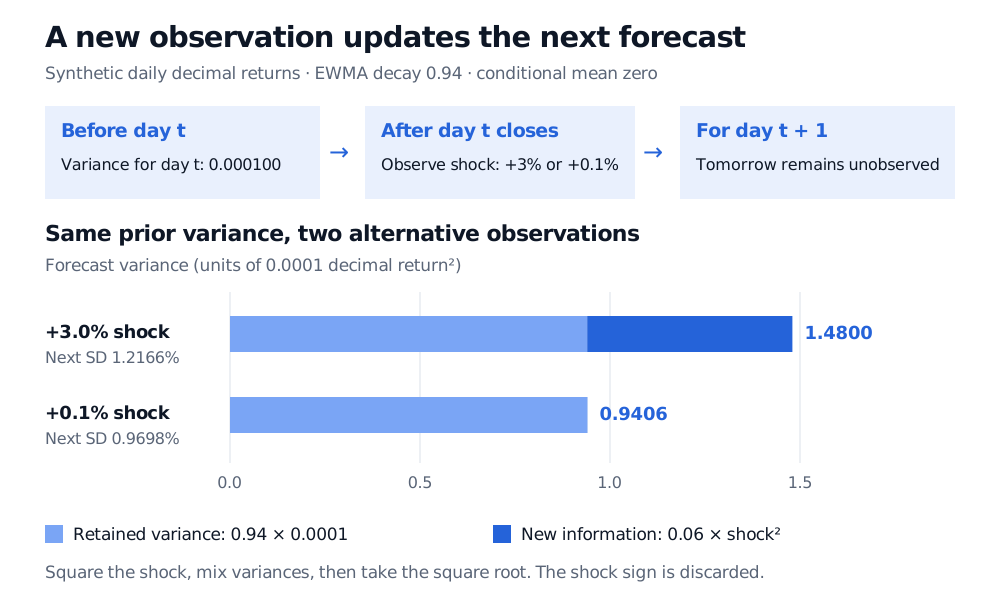
Suppose the desk had assigned today a daily variance of 0.0001, corresponding to 1% standard deviation, and today’s demeaned return is +3%. Then
Averaging the two standard deviations directly would give 0.94(1%)+0.06(3%)=1.12%, a different calculation. The squared shock is the new information entering this model. A −3% shock produces exactly the same update; EWMA alone cannot represent asymmetric responses to good and bad news.
If the observed shock had instead been +0.1%, the next variance would be 0.00009406, with standard deviation 0.9698%. The model revises risk downward because that squared shock is below the previous variance estimate.
EWMA information timeline: before day t, its forecast variance is 0.000100. After observing a hypothetical +3% shock, retained variance 0.000094 plus news 0.000054 gives next variance 0.000148 and daily standard deviation 1.2166%. An alternative +0.1% shock gives variance 0.00009406 and standard deviation 0.9698%.
Original synthetic example with zero conditional mean. The two rows are alternative observations from the same prior state, not successive days. Bar lengths are variance, in units of 0.0001 decimal return squared.
The timing matters as much as the arithmetic. Today’s +3% return updates tomorrow’s forecast. It cannot improve the forecast already issued for today. Initial variance, mean estimates and decay selection must also use data available at their respective forecast times. Updating the state with new data is legitimate; choosing the model after inspecting its final test results changes the experiment. This is a common route to look-ahead bias.
A forecast for day 20 is not a forecast for 20 days
EWMA has no separate long-run variance anchor. Under its zero-mean conditional return model, the expected future daily variance stays at the latest forecast when projected from a fixed information date. Actual future shocks will still change the state.
A basic GARCH(1,1) model adds an intercept:
ht+1=ω+αϵt2+βht.
With unit-variance innovations, ω>0, α,β≥0 and p=α+β<1, its finite long-run variance is hˉ=ω/(1−p). Conditional daily variance forecasts obey
ht+k∣t=Emodel[ht+k∣Ft]=hˉ+pk−1(ht+1−hˉ),k≥1.
This is mean reversion in the variance forecast, not a promise about each realised path. It is one way to model volatility clustering. Fitted parameters and the initial state introduce estimation uncertainty beyond the formula.
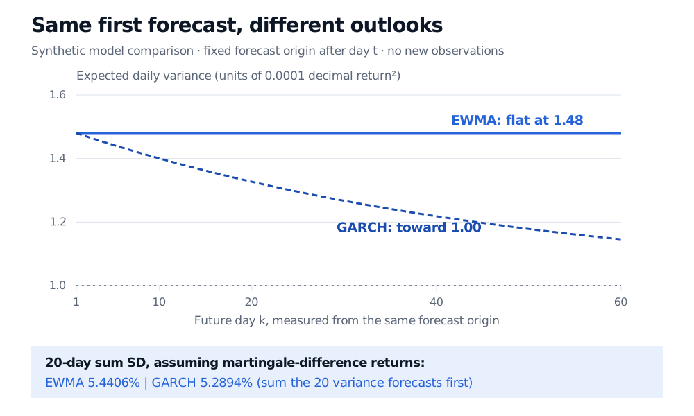
Choose synthetic parameters ω=0.000002, α=0.06 and β=0.92. With the same prior variance and +3% shock, GARCH also gives 0.000148 tomorrow, but its long-run variance is 0.0001 and its later forecasts decline toward that level. Equal next-day forecasts need not imply equal risk over a longer holding period.
For zero-mean martingale-difference log returns, the model makes future returns conditionally uncorrelated at a fixed origin. Consequently,
Varmodel(k=1∑HRt+k∣Ft)=k=1∑Hht+k∣t.
Sum the forecast variances and then take the square root. In this example the 20-day cumulative log-return standard deviation is 5.4406% under EWMA, versus 5.2894% under GARCH. These are dispersions over the whole interval; neither is the daily volatility forecast for day 20.
Fixed-origin expected daily variances from two hypothetical models start at 0.000148. EWMA stays flat; GARCH with omega 0.000002, alpha 0.06 and beta 0.92 declines toward 0.0001. Summing 20 daily variance forecasts gives cumulative log-return standard deviations of 5.4406% for EWMA and 5.2894% for GARCH under zero conditional cross-covariances.
Original synthetic model comparison. These are conditional expectations from one forecast origin, not simulated variance paths. The long-run line is a model parameter, not an observed market constant.
Outside those assumptions, include the relevant conditional covariance terms. A constant daily variance times H requires a flat variance forecast as well as zero cross-covariances. Annualising a daily number by 252 is a stated scaling convention; it is not, by itself, a fitted one-year forecast. Compounded simple-return risk requires its own treatment.
Taking a square root changes a forecasting target
Tomorrow’s ht+1 is known from today’s state within these models, so ht+1 is their next-day conditional standard deviation. Farther ahead, the variance state is random. In general,
Emodel[ht+k∣Ft]≤Emodel[ht+k∣Ft].
This follows from Jensen’s inequality. For a separate two-state illustration, suppose a future daily variance is equally likely to be 0.0001 or 0.0009. Expected daily standard deviation is 2%, whereas the square root of expected daily variance is 2.2361%. Both quantities are legitimate; they answer different questions. Label the right-hand quantity as a square-root variance forecast rather than silently calling it expected future volatility.
Judge the forecast against the right later observation
A single small return does not disprove a high variance forecast. With a correctly specified conditional mean, tomorrow’s squared residual is a conditionally unbiased but noisy variance proxy. Intraday realised variance can provide a richer measurement, but its coverage and sampling must match the target; it does not automatically recover every conditional-variance object.
For a variance proxy y and positive forecast h, two common scores are variance squared error (y−h)2 and the QLIKE-related score
Evaluate chronologically on data kept separate from model selection, retain simple benchmarks, and account for dependent score differences—especially with overlapping horizons. A good variance score also does not establish accurate tail probabilities: Value at Risk requires more of the return distribution than its variance.
For a deeper walkthrough, the public EWMA forecasting article develops initialisation, decaying weights and the append-before-update forecasting clock. The public forecast-evaluation article follows the noisy-target and chronological-testing decisions in more detail.
Sources
John C. Hull, Options, Futures, and Other Derivatives, 9th Global Edition, §23.2 (EWMA, equation 23.7), §23.3 (GARCH) and §23.6 (future variance forecasts, equation 23.13). Numerical examples and figures here are original.