Triangular matrix: Definition & Examples

A triangular matrix is a square matrix with zeros everywhere on one side of its main diagonal. A lower triangular matrix has zeros above the diagonal; an upper triangular matrix has zeros below it. The diagonal itself may contain zeros.

The practical payoff is an order in which to solve a system of linear equations: one unknown at a time. Risk calculations use triangular factors both to solve systems and to build correlated return shocks.

For example,

L=\begin{pmatrix}2&0\\1&3\end{pmatrix}, \qquad U=\begin{pmatrix}2&1\\0&3\end{pmatrix}

are lower and upper triangular, respectively. Here

U=L^\top

: a transpose reverses the triangular orientation. Neither matrix is diagonal or symmetric. A diagonal matrix is both lower and upper triangular.

Solve in the direction the zeros allow

Suppose a hypothetical exposure model has two instruments. Per unit held, instrument 1 contributes 2 units of exposure A and 1 unit of exposure B; instrument 2 contributes no A and 3 units of B. To reach targets of 4 units of A and 8 units of B, the holdings solve

L\mathbf{x}=\mathbf{b}, \qquad \begin{pmatrix}2&0\\1&3\end{pmatrix} \begin{pmatrix}x_1\x_2\end{pmatrix} =\begin{pmatrix}4\\8\end{pmatrix}.

The first row contains only $x_1$ , so $2x_1=4$ gives $x_1=2$ . Substitute that into the second row:

x_2=\frac{8-x_1}{3}=\frac{8-2}{3}=2.

This is forward substitution: work from the first row down. Checking the original targets gives

2(2)=4

and

1(2)+3(2)=8

. This toy model matches only its two stated exposures; it says nothing about cost, funding, omitted risks or whether the holdings are permitted.

For a general lower triangular matrix with nonzero diagonal, the same rule is

x_i=\frac{b_i-\sum_{j=1}^{i-1}L_{ij}x_j}{L_{ii}}, \qquad i=1,\ldots,n.

The sum is empty when $i=1$ . All the unknowns needed for row $i$ have already been found.

For an upper triangular system, start at the last row and move up: back substitution. With

U

above and a different target

(6,6)^\top

, first solve

3x_2=6

, then

2x_1+x_2=6

. Again the solution is

(2,2)^\top

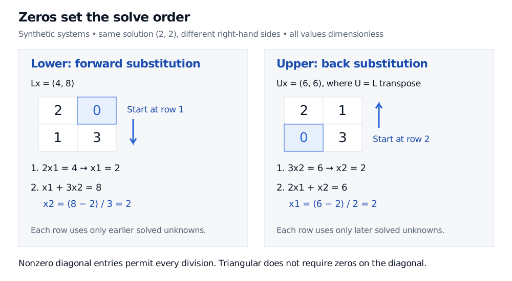
Lower triangular L has rows 2,0 and 1,3. With target (4,8), solve x1=2 before x2=2. Upper triangular U has rows 2,1 and 0,3. With target (6,6), solve x2=2 before x1=2. The two targets differ.

Original synthetic systems, with dimensionless coefficients and targets for comparison. The highlighted zeros determine which unknown can be solved first. Transposing the matrix changes the system, so the right-hand side also differs here.

A dense triangular solve takes

O(n^2)

arithmetic work. That is why algorithms often factor a more complicated matrix once and reuse its triangular factors for many targets. There is no need to form an explicit matrix inverse just to solve each system. Easy substitution does not guarantee an accurate answer when the system is poorly conditioned.

The diagonal gives two shortcuts

For either triangular orientation, the determinant is the product of the diagonal entries:

\det(T)=\prod_{i=1}^{n}T_{ii}.

Thus

\det(L)=2\times3=6

. A triangular matrix is invertible if and only if every diagonal entry is nonzero. If one is zero, the matrix is still triangular, but some right-hand sides have no solution and the solvable ones have nonunique solutions. Dividing by zero is not a way to continue substitution.

Its eigenvalues, counted with multiplicity, are also the diagonal entries:

T-\lambda I

stays triangular, so its determinant is

\prod_i(T_{ii}-\lambda)

. The eigenvalues of

L

are therefore 2 and 3.

These are not generally its singular values. Those depend on

L^\top L

, which here is

L^\top L=\begin{pmatrix}5&3\\3&9\end{pmatrix}.

Its eigenvalues are $7+\sqrt{13}$ and $7-\sqrt{13}$ , so the singular values of $L$ are their positive square roots. Also, reducing a general matrix to triangular form by ordinary row elimination preserves its solutions when the right-hand side is transformed consistently, but generally changes its eigenvalues. You cannot read the original matrix's eigenvalues from those pivots.

A triangular factor can create covariance

Consider a separate synthetic return model over one fixed horizon. Let $\mathbf{z}$ have mean zero and covariance matrix $I$ , and set centred decimal returns to $\mathbf{R}=C\mathbf{z}$ , where

C=0.1L=\begin{pmatrix}0.2&0\\0.1&0.3\end{pmatrix}.

Then $R_1=0.2z_1$ and $R_2=0.1z_1+0.3z_2$ . The first shock feeds both returns; the second feeds only the second return. Their population covariance is

\Sigma=CIC^\top=CC^\top =\begin{pmatrix}0.04&0.02\\0.02&0.10\end{pmatrix}.

The entries of

C

convert dimensionless shocks to decimal returns; entries of

\Sigma

are in squared decimal-return units. The second variance is

0.1^2+0.3^2=0.10

, not just the square of the second diagonal entry. The triangular factor is not itself the covariance matrix.

This is the structure used by Cholesky decomposition. A real symmetric positive definite matrix has a unique lower triangular Cholesky factor with positive diagonal. An arbitrary triangular matrix need not have a positive diagonal, and a singular covariance does not admit that strictly positive-diagonal factor. The covariance identity requires uncorrelated unit-variance shocks; assuming independent standard normal shocks additionally makes these returns jointly normal. A finite simulated sample will generally have a covariance different from the population target.

For the construction and its use in two successive triangular solves, see Cholesky Factorisation. The full lesson requires membership, with a public preview.

Sources

Gilbert Strang, Introduction to Linear Algebra, 5th edition (2016), §2.2, worked example 2.2B, and §2.6: triangular systems, nonzero pivots and forward/back substitution. §6.1, “Introduction to Eigenvalues,” p. 294 explains triangular eigenvalues and why elimination generally changes eigenvalues.
Lloyd N. Trefethen and David Bau III, Numerical Linear Algebra (SIAM, 1997), Lecture 17, Algorithm 17.1 and equation (17.2), on successive substitution and its operation count; Lecture 23, Theorem 23.1, on Cholesky factorisation.
LAPACK Users' Guide, “Linear Equations”: triangular substitution and the triangular factors used in LU and Cholesky methods.

The exposure model, return model and diagram are original hypothetical examples.

Solve in the direction the zeros allow

The diagonal gives two shortcuts

A triangular factor can create covariance

Sources

Related terms

Determinant

Diagonal matrix

Eigenvalue

Matrix

Matrix inverse

Matrix transpose

Positive definite matrix

Singular value

System of linear equations