Singular value: Definition & Examples

A singular value is a nonnegative principal stretch factor of a matrix. It measures how much the matrix changes length along a particular input direction, using Euclidean norms. A small singular value identifies a direction that produces little observable output. Recovering a position or model parameter along that direction can therefore magnify measurement error.

The singular value decomposition chooses orthonormal input directions $\mathbf v_i$ and output directions $\mathbf u_i$ so that

A\mathbf v_i=\sigma_i\mathbf u_i, \qquad \sigma_1\ge\sigma_2\ge\cdots\ge0.

Both direction vectors have length one, so

\lVert A\mathbf v_i\rVert_2=\sigma_i

. The directions need not coincide, and the input and output spaces can even have different dimensions. Unlike an eigenvalue, a singular value is defined for rectangular matrices and never carries a negative sign.

Two controls, three reported exposures

Suppose a risk desk uses two position controls and reports three factor exposures. For this synthetic example, each position is divided by its chosen reference position size; each exposure is divided by its chosen reference exposure size. Thus

\mathbf x

and

\mathbf b=A\mathbf x

are dimensionless normalised coordinates, with the following illustrative map:

A=\begin{pmatrix}3&0\\0&1\\0&0\end{pmatrix}, \qquad \begin{pmatrix}b_1\b_2\b_3\end{pmatrix} = \begin{pmatrix}3x_1\x_2\\0\end{pmatrix}.

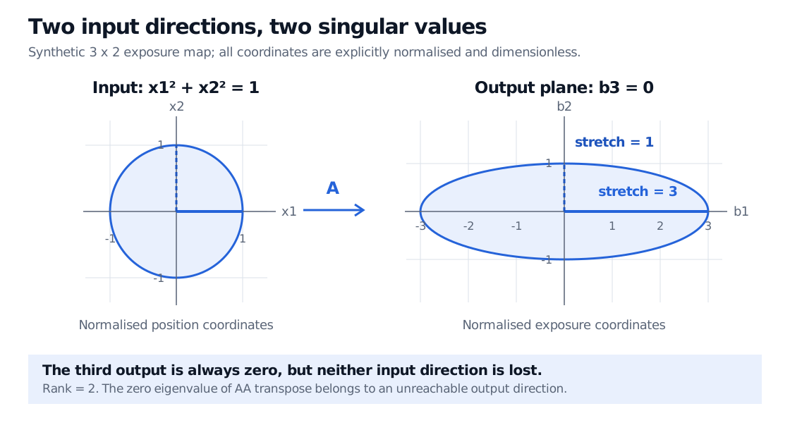
A unit change in the first control gives output $(3,0,0)$ , of length $3$ . A unit change in the second gives $(0,1,0)$ , of length $1$ . These are orthogonal output directions, so the singular values are $3$ and $1$ .

All unit-length input combinations form a circle. Their images form an ellipse in the plane $b_3=0$ , with semiaxes $3$ and $1$ :

x_1^2+x_2^2=1 \quad\Longrightarrow\quad \left(\frac{b_1}{3}\right)^2+b_2^2=1, \qquad b_3=0.

A synthetic dimensionless 3 by 2 map sends a unit circle of position changes to an ellipse in the b3 equals zero output plane. Horizontal and vertical semiaxes are 3 and 1. There are two positive singular values and rank is 2 despite the unreachable third output direction.

Original synthetic exposure map. Equal scale on the two axes within each panel; the output is shown in its $b_3=0$ plane. The semiaxis lengths are the singular values $3$ and $1$ .

This is geometry in the specified normalised coordinates. It does not say that an exposure's Euclidean length is portfolio volatility, or that these positions meet funding or trading constraints.

Why the extra zero is not a lost input

The usual singular-value list of an

m\times n

matrix contains

\min(m,n)

values, counting multiplicity and including zeros. Here there are two. Using the transpose,

A^\top A=\begin{pmatrix}9&0\\0&1\end{pmatrix}, \qquad AA^\top=\begin{pmatrix}9&0&0\\0&1&0\\0&0&0\end{pmatrix}.

For a tall matrix, the singular values are the square roots of the eigenvalues of $A^\top A$ : here $\sqrt9=3$ and $\sqrt1=1$ . More generally, take the largest $\min(m,n)$ eigenvalues of $A^\top A$ ; a wide matrix has additional structural zeros in that larger Gram matrix.

Both products are positive semidefinite: for example,

\mathbf z^\top A^\top A\mathbf z=\lVert A\mathbf z\rVert_2^2\ge0

. This guarantees nonnegative eigenvalues and real square roots.

The zero eigenvalue of

AA^\top

describes the third output direction, which these controls cannot reach. It does not imply a nonzero input is mapped to zero. The two columns are independent, the rank is

2

, and the input null space contains only zero. Every reachable exposure target has a unique pair of controls; arbitrary three-dimensional targets need not be reachable.

A weak direction makes the reverse problem fragile

Now replace the second loading by $0.001$ :

B=\begin{pmatrix}3&0\\0&0.001\\0&0\end{pmatrix}.

Its singular values are $3$ and $0.001$ . Its rank is still exactly $2$ , but recovering the second control requires $x_2=b_2/0.001=1000b_2$ .

Take the reachable target $\mathbf b=(3,0,0)$ , which gives $\mathbf x=(1,0)$ . An exposure measurement error $\delta\mathbf b=(0,0.001,0)$ changes the inferred controls to $(1,1)$ . An absolute output error of $0.001$ has produced an absolute control error of $1$ : amplification by $1000$ .

The Euclidean condition number of this full-column-rank map is

\kappa_2(B)=\frac{\sigma_{\max}}{\sigma_{\min}} =\frac{3}{0.001}=3000.

That is a relative sensitivity measure. In this particular example, the relative target error is

0.001/3=1/3000

, while the relative control error is

1/1=1

. The relative amplification attains

3000

; other error directions can produce much smaller changes. A numerical rank calculation may treat the weak direction as zero only under a stated tolerance; that is a modelling or numerical decision, distinct from exact rank.

The scaling convention matters throughout. Multiplying the whole matrix by a nonzero scalar multiplies every singular value by its absolute value, leaving their ratio unchanged. Rescaling individual inputs or outputs can change that ratio. A matrix mixing raw dollars and basis points needs an explicit metric or normalisation before its principal stretches have a useful economic interpretation.

For the derivation of the fixed-matrix sensitivity bound in a square system, read Condition Numbers. Its public page is a preview; the full lesson requires membership.

Sources

Gilbert Strang, Introduction to Linear Algebra, 5th ed. (Wellesley-Cambridge Press, 2016), §7.2, “Bases and Matrices in the SVD,” especially $A\mathbf v_i=\sigma_i\mathbf u_i$ and the construction from $A^\top A$ .
MIT OpenCourseWare: Gilbert Strang, Lecture 29 — Singular value decomposition — the two orthogonal bases and rectangular factorisation.
University of Illinois CS357: Singular Value Decomposition — singular-value counts, rank, Euclidean matrix norms and the pseudoinverse.

Two controls, three reported exposures

Why the extra zero is not a lost input

A weak direction makes the reverse problem fragile

Sources

Related terms

Eigenvalue

Euclidean norm

Matrix

Matrix rank

Matrix transpose

Null space

Positive semidefinite matrix