A Markov process forecasts from its current state. Separate state, filtration and homogeneity, then see how merging states can make history predictive again.
Markov process
A Markov process is a stochastic process whose current state contains all the information from the specified past that is needed to determine its future conditional distribution. Once that state is known, earlier history supplies no further predictive information under the model.
For a quant, the choice of state is the important part. A model may need today's price alone, or it may need a vector containing price, volatility and other variables. A compact Markov state can make forecasting, simulation and derivative valuation manageable. Calling a single price series Markov is a substantive restriction on its dynamics, not a consequence of recording the latest price.
State, time and available information
Let Xt be the state at time t, and let the filtrationFt represent the information available by then. The state must be observable within that information: formally, Xt is Ft-measurable. The Markov property, relative to this filtration, can be written
P(Xu∈A∣Ft)=P(Xu∈A∣Xt),u>t,
almost surely, for every measurable set of states A. The right side is a conditional probability, not an unconditional forecast. On the usual finite or Euclidean state spaces, a transition kernelKt,u(x,A) describes that conditional law as a function of the present state x. The calendar times remain known. Pitman's Berkeley notes formulate the discrete-time version using kernels and distinguish it from homogeneity.
The natural choice is the natural filtration, generated by the process's observations up to t. A larger information set can change the answer. For example, revealing a future value in advance can invalidate a property that held using only past observations. “Markov” must therefore be understood with its state, information set and probability law specified. A claim under a physical forecasting law does not automatically establish the same claim under a different pricing law.
Two other distinctions prevent common misreadings:
Markov does not mean independent. The current state can strongly affect the future. The restriction concerns the extra value of older history after conditioning on the present. It does not require independent and identically distributed variables.
Markov does not mean time-homogeneous. Homogeneity adds that the transition law depends on elapsed time, rather than on the starting calendar date separately. A known seasonal transition rule can still be Markov.
A daily regime forecast
Consider a hypothetical model with states Calm (C) and Stress (S). Stipulate the same one-day transition matrix each day, with rows and columns ordered (C,S):
P=(0.800.300.200.70).
Each row describes tomorrow conditional on today; its entries are nonnegative and sum to one. This is a finite, discrete-time, time-homogeneous Markov chain, one particular Markov process. Its probabilities are teaching assumptions, not calibrated market estimates.
If today is Stress, tomorrow is Calm with probability 30%, whether the earlier observed regimes were Calm or Stress, provided the history being conditioned on has positive probability. If today is Calm, tomorrow is Calm with probability 80%. Dependence on today's regime is perfectly compatible with the Markov property.
Starting definitely in Calm, a two-day Stress forecast combines two disjoint paths:
Route
Probability
Calm → Calm → Stress
0.80×0.20=0.16
Calm → Stress → Stress
0.20×0.70=0.14
Stress on day 2
0.16+0.14=0.30
Equivalently, the row-vector calculation is (1,0)P2=(0.70,0.30). The calculation uses both the Markov restriction and the stipulated homogeneous transitions. A fitted one-day table alone does not prove that real regime histories satisfy either assumption. Nor does a 30% Stress probability specify a loss amount; a risk calculation also needs the loss distribution conditional on each regime.
For transition diagrams and the construction of a state that retains recent history, the Markov Chains — Transition Matrices and the Markov Property lesson develops this finite-state case further. The full lesson requires membership; a public preview is available.
Why a projection can lose the property
A function of a Markov process need not be Markov. Merging distinct states can discard information needed to choose the next transition law.
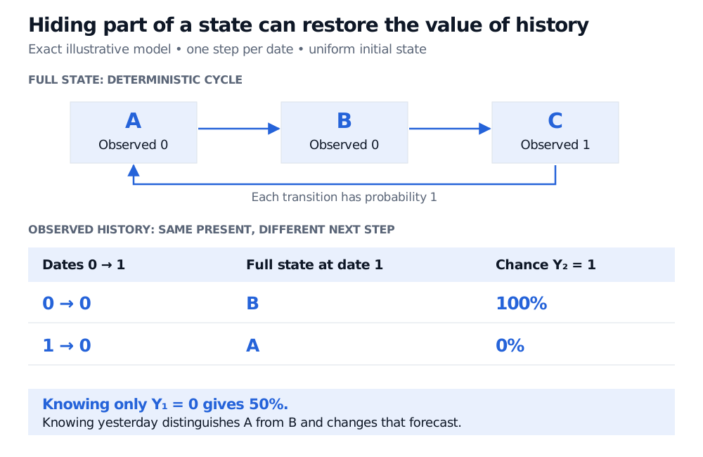
Here is an exact counterexample, separate from the regime model. A process Zn cycles deterministically through A→B→C→A, starting uniformly in the three states. The full state is Markov: its current value determines its next value. Now observe only Yn, equal to 0 in states A and B, and 1 in state C.
At date 1, the observation Y1=0 leaves A and B equally likely, so
P(Y2=1∣Y1=0)=21.
But yesterday's observation resolves the ambiguity:
P(Y2=1∣Y0=0,Y1=0)P(Y2=1∣Y0=1,Y1=0)=1,=0.
The first history must come from A→B→C; the second from C→A→B. Both histories have probability 1/3. Older information changes the forecast even though the current observation is identical. Thus Y fails the Markov property in its own natural filtration.
A deterministic cycle A to B to C to A is Markov. Observing A and B as 0 and C as 1 loses information. With a uniform initial state, histories 0 to 0 and 1 to 0 both end at observed 0 but give next-1 probabilities 100% and 0%; knowing only current 0 gives 50%.
Exact illustrative three-state model. All three initial states have probability 1/3. Merging A and B makes past observations useful for predicting the next one.
The same question arises when retaining only price from a richer price-and-volatility state. The joint state may be Markov while price alone is not; one must check whether the omitted variable changes the forecast. Conversely, an invertible transformation retains the current state's information and preserves Markovianity, with the calendar time included when the transformation depends on time.
Beyond a finite table
Time and state space are separate choices. A continuous-time Markov chain can jump among discrete states. Brownian motion has continuous time and continuous state space. With its natural filtration, its future increment is independent of the past, so
Wt+h∣Ft∼N(Wt,h),h>0.
The current level determines the conditional mean; elapsed time determines the conditional variance. Lalley's Brownian-motion lecture, §§4 and 6, develops this transition law and the filtration argument. Brownian levels themselves are not independent observations.
A Markov state also need not contain every quantity needed to value a contract. Even with a Markov price model, an Asian payoff depends on an accumulated average. A pricing state may therefore need to include that accumulated quantity. And the property at fixed times should not be silently extended to random observation times: that extension is the strong Markov property.
Sources
John C. Hull, Options, Futures, and Other Derivatives, ninth Global Edition (Pearson, 2018), §14.1: Markov modelling and the conditional distribution of future prices.
Richard Durrett, Essentials of Stochastic Processes, third edition (2016), §§1.1–1.2 and §4.1: discrete- and continuous-time chains, homogeneous transition laws and multistep probabilities.
Steven P. Lalley, Lecture 5: Brownian Motion, University of Chicago, §§4 and 6: Brownian transition probabilities and the Markov property relative to its natural filtration.