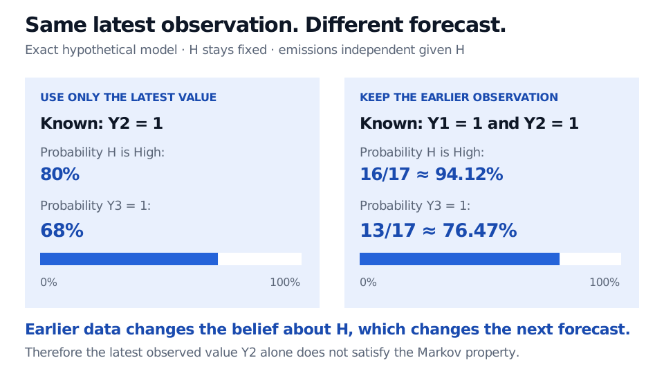
The Markov property is a claim about what the current state retains. Compare exact forecasts of 68% and 76.47% when an earlier reading reveals information about a hidden regime.
Markov property
The Markov property says that the current state contains all the information from the specified past needed to determine the conditional distribution of the future. Once the current state is known, older information adds nothing to that forecast.
For a quant, the critical word is state. Today's credit rating, price or volatility estimate may be convenient to record without being enough to predict tomorrow's risk. A model can have the Markov property in a richer state while a single observed component fails it.
The equality to check
Let Xt be a stochastic process, and let Ft be a filtration: the information available by time t. Assume Xt is observable from that information. The process has the Markov property relative to this filtration if, for every measurable state set A and fixed times s<t,
P(Xt∈A∣Fs)=P(Xt∈A∣Xs)almost surely.
The equality concerns the whole conditional distribution, not just its mean. Matching an expected return while allowing past returns to predict the next period's volatility does not establish the Markov property. This is a conditional independence statement: the current state screens off the specified past when forecasting the future. Drapeau's notes give the distributional definition and its equivalent formulation using expectations of all bounded measurable functions.
When no larger information set is specified, the usual choice is the natural filtration, FsX=σ(Xu:u≤s), containing the process's own observed history. A claim relative to that history need not survive adding information that reveals future outcomes. The filtration is part of the claim; Norris's Section 3.3 explicitly distinguishes these cases.
For a discrete Markov chain, the next-step version is
P(Xn+1=j∣X0=i0,…,Xn=i)=P(Xn+1=j∣Xn=i),
for conditioning histories with positive probability. Requiring this at every step also gives the corresponding finite-future distributional statement. It does not require the right-hand side to be independent of n: a time-homogeneous model adds that restriction. Nor must successive states be independent or identically distributed.
A small example that works is a simple random walk. Start at S0=0 and add independent fair increments of +1 or −1. Given S1=1, the next state is 0 or 2, each with probability 1/2. More generally, the next independent increment moves the current state up or down; older positions cannot improve that forecast under this model. The positions themselves remain dependent.
When the latest observation loses information
Consider a hypothetical risk indicator Yn, where 1 means a high reading and 0 a low reading. At the outset, an unobserved regime H is chosen, High or Low, each with probability 1/2. It stays fixed. Conditional on H, the daily readings are independent, with
P(Yn=1∣H=High)=0.8,P(Yn=1∣H=Low)=0.2.
These are stipulated probabilities, not fitted market estimates. Conditional independence of the readings given H does not make them independent when H is hidden: repeated high readings provide accumulating evidence about the same persistent regime.
Suppose we retain only today's reading, Y2=1. Bayes' theorem gives an 80% probability of High, so tomorrow's forecast is
P(Y3=1∣Y2=1)=0.8(0.8)+0.2(0.2)=0.68.
Now keep yesterday's reading too: Y1=1,Y2=1. The probability of High becomes
Both forecasts have latest reading Y2 equal to 1. Using only Y2 gives an 80% probability of the High regime and a 68% chance of Y3 equal to 1. Retaining Y1 equal to 1 raises those values to 16/17, about 94.12%, and 13/17, about 76.47%.
Exact probabilities in a hypothetical persistent-regime model. Both information sets include the same latest reading; the earlier reading changes the forecast through the belief about the hidden regime.
The two forecasts differ even though the latest observation is identical. Therefore the observed sequence Yn fails the first-order Markov property relative to its own history. This is a counterexample, not a claim that every process with a hidden state produces non-Markov observations. If the two emission probabilities were equal, for example, the readings in this construction would be independent.
Retain what the forecast needs
Knowing the true H would make predicting the readings straightforward, but an analyst does not observe it. In this particular model, a usable alternative state is the current belief
πn=P(H=High∣Y1,…,Yn).
It gives P(Yn+1=1∣Y1,…,Yn)=0.2+0.6πn. After the next reading, Bayes' rule updates the belief using only πn and that new reading. Thus the belief process has a Markov description; discarding everything except the latest binary reading did not. The richer state is justified by the model's conditional independence, rather than by a rule that any short history must suffice.
This is why state choice matters in credit migration and regime modelling. A transition table indexed only by today's label pools histories that may imply different forecasts. More detailed states can preserve useful information, at the cost of more quantities to estimate. The SelfMadeQuant lesson Markov Chains — Transition Matrices and the Markov Property develops credit-rating states and finite-history state expansion (membership for the full lesson; public preview).
A related pricing distinction is that a Markov price process does not make a path-dependent contract depend only on today's price. A running maximum or accumulated average may also belong in the valuation state. The modelling task is to retain the information required for the particular future distribution or payoff being computed.
Sources
Richard Durrett, Essentials of Stochastic Processes, third edition, Springer, 2016, Section 1.1. Defines discrete-time chains and explicitly identifies time homogeneity as an additional restriction.
Samuel Drapeau, Stochastics: Markov Processes. Measurable-state definition, natural filtration and conditional-distribution formulation.
James Norris, Advanced Probability, Section 3.3. Natural-history versus specified-filtration Markov chains.
Steven E. Shreve, Stochastic Calculus and Finance, Carnegie Mellon lecture notes prepared by Prasad Chalasani and Somesh Jha, 25 July 1997, Sections 4.1–4.3. Markov structure, conditional distributions and the distinction between European and path-dependent claims.