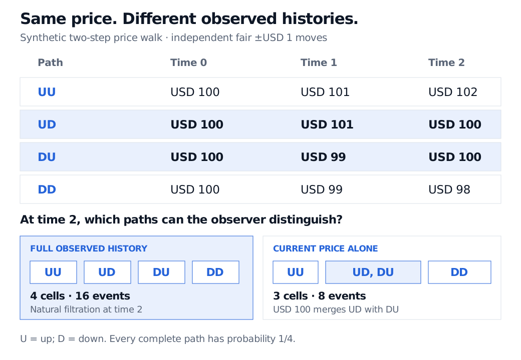
A natural filtration records a process’s entire observed history. A two-step price walk shows why the current price can contain less information than the path.
Natural filtration
The natural filtration of a stochastic process is the information generated by observing that process's entire history up to each time. For a price process, it lets a trading rule use previously observed prices as well as today's price. A price returning to yesterday's level does not erase what the trader saw in between.
For a real-valued process X on a probability space, its raw natural filtration is
FtX=σ(Xs:0≤s≤t).
The symbol σ(⋅) means the smallest sigma-algebra making all the listed observations measurable. In discrete time this becomes FnX=σ(X0,…,Xn). The time index matters: observations after t are absent.
This is a filtration because extending the observed history preserves earlier information. It is also the smallest filtration to which X is an adapted process. To see why, suppose another filtration (Gt) makes X adapted. For every s≤t, Xs is measurable with respect to Gs⊆Gt. Therefore all observations generating FtX are measurable with respect to Gt, giving FtX⊆Gt.
Returning to USD 100 does not reset the history
Take an original synthetic two-step price model, with prices measured in USD:
S0=100,S1=100+ξ1,S2=100+ξ1+ξ2.
The increments ξ1,ξ2 are independent, each taking +1 or −1 with probability 1/2. Label the four complete paths UU,UD,DU,DD, where U means an up move and D a down move. Each path has probability 1/4.
The natural information partitions are:
Observation time
Paths still indistinguishable
0
{UU,UD,DU,DD}
1
{UU,UD} and {DU,DD}
2
{UU}, {UD}, {DU} and {DD}
Each cell is an atom of the finite sigma-algebra; its events are all unions of cells. The natural sigma-algebras therefore contain 2, 4 and 16 events at times 0, 1 and 2. The initial information is trivial here because S0 is constant. A random initial value would already reveal information at time zero.
Now compare two paths:
UD gives the observed sequence USD 100, USD 101, USD 100.
DU gives the observed sequence USD 100, USD 99, USD 100.
At time 2, the current price is USD 100 on both paths. Observing only S2 cannot distinguish them, but observing (S0,S1,S2) can. Indeed, the increments can be recovered from consecutive observed prices.
Four equally likely paths from USD 100: UU ends at USD 102, UD and DU both end at USD 100 after different intermediate prices, and DD ends at USD 98. The full history separates four cells and 16 events; current price alone separates three cells and eight events.
Original synthetic finite-state example. The shaded rows finish at the same price but have different observed histories. Boxes below show distinguishable information cells; each sigma-algebra contains every union of its cells.
Thus σ(S2) has only three atoms, corresponding to USD 98, USD 100 and USD 102, and eight events. In particular,
σ(S2)⊊F2S.
Replacing the natural filtration with (σ(St)) need not even produce a filtration. Here the event “the first move was up,” {UU,UD}, is known at time 1 but cannot be reconstructed from S2 alone. The replacement would forget information already observed.
Why a path-dependent payoff needs that distinction
Consider a terminal payment A of USD 6 if the first move was up, and zero otherwise. On the four paths its values are (6,6,0,0) USD. The natural history tells the observer the eventual payment as soon as the first move is observed.
At time 2, conditioning only on a current price of USD 100 mixes the equally likely paths UD and DU. Their payments average to USD 3:
E[A∣S2=100]=21(6)+21(0)=3.
By contrast, E[A∣F2S]=A: the full observed history distinguishes the USD 6 payment on UD from the zero payment on DU. These are conditional payment forecasts, without discounting or a pricing claim.
The Conditional Expectation lesson develops the averaging machinery and explains why a forecast is itself a random variable. Its public page is a preview; the full lesson requires membership.
Calling this filtration “natural” imposes no Markov property. A Markov model permits certain forecasts of future states to depend only on the present state; that is a property of its conditional laws. Even in such a model, the natural filtration retains the past, and a payoff depending on that past can require more than the current state.
Raw history, additional signals and augmentation
The natural filtration is tied to the named process. Observing a price alone need not reveal an earnings announcement, another asset's price or a latent volatility factor. A larger market filtration can include such observations. Whether a rule is admissible, or a process is a martingale, must be assessed relative to the specified information and probability measure.
In continuous time, check the convention before using a theorem. The raw natural filtration above is not automatically complete or right-continuous. Completion puts all subsets of ambient probability-zero events into the information sets. Right-continuity requires
Ft=u>t⋂Fu.
An augmentation imposing both is commonly called the usual augmentation. It can enlarge the raw natural filtration; do not silently identify the two. Completion depends on the probability measure, whereas the raw generated sigma-algebras are defined by the observation maps. The finite example needs no such augmentation: every complete path has positive probability, and time takes just the values 0, 1 and 2.
Sources
Steven E. Shreve, Stochastic Calculus and Finance, CMU lecture notes prepared by Prasad Chalasani and Somesh Jha, 25 July 1997, §1.2, Definition 1.3 and Example 1.3: finite information, generated sigma-algebras and the distinction between observing a price and observing its history. The example and figure here are original.