Markov chain: Definition & Examples

A Markov chain is a sequence of random states in which the conditional distribution of the next state depends on the current state, with no additional dependence on earlier states once the current state is known. It is a particular kind of stochastic process, usually studied on a finite or countable state space.

For a risk model, the useful question is: what information must the current state contain to forecast the next step? A credit rating or a market-regime label can serve as a state. Calling its evolution Markov is a modelling assumption about information; a row of probabilities does not establish that the assumption holds in data.

What the current state tells you

In discrete time, write the state on day $n$ as $X_n$ . The Markov property says

\mathbb{P}(X_{n+1}=j\mid X_n=i,X_{n-1}=i_{n-1},\ldots,X_0=i_0) =\mathbb{P}(X_{n+1}=j\mid X_n=i),

for histories with positive probability. The point is the conditioning: older observations add no information after the current state has been supplied. Conditional probability is doing the work here.

This does not mean successive states are independent. If stress tends to persist, knowing that today is stressed changes tomorrow's forecast. Nor does the property require a constant transition rule. A time-homogeneous chain adds that assumption: its one-step probabilities do not depend on the day. The example below uses this additional restriction. Stanford's Markov-chain notes develop the conditional-state interpretation and multistep matrix calculation.

Choosing the state is consequential. If tomorrow's risk depends on both today's regime and how long it has lasted, a two-label calm/stress model may fail the Markov property. A richer state, such as the pair of the last two labels when dependence is limited to two days, can retain the relevant history. More states also require more transition probabilities to estimate.

A risk forecast with two possible regimes

Suppose a hypothetical daily model has states Calm (

C

) and Stress (

S

). These labels and probabilities are stipulated for teaching; they are not estimated market regimes. Use the row convention for the transition matrix: row

i

describes tomorrow conditional on today being

i

P=\begin{pmatrix}0.90&0.10\\0.20&0.80\end{pmatrix}, \qquad P_{ij}=\mathbb{P}(X_{n+1}=j\mid X_n=i).

The state order is

(C,S)

for both rows and columns. From Calm, tomorrow is Stress with probability 10%; from Stress, that probability is 80%. This state dependence makes the distinction from independence concrete. Each entry is nonnegative and each row sums to one. The probabilities refer to one day: applying this same matrix to a different time interval silently changes the model.

Let $q_n$ be the row vector containing the probabilities of the two states on day $n$ . Then

q_{n+1}=q_nP,\qquad q_n=q_0P^n.

A model needs an initial distribution as well as its transition rule. Starting in Calm means $q_0=(1,0)$ , so $q_1=(0.90,0.10)$ . One more step gives

q_2=(0.90,0.10)P=(0.83,0.17).

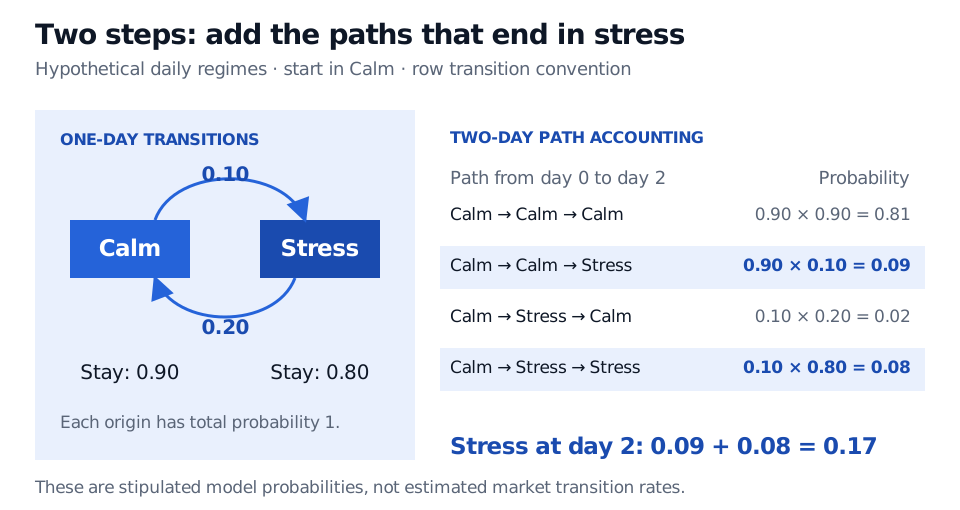
Where does the 17% come from? There are two disjoint ways to end in Stress: Calm → Calm → Stress, with probability $0.90\times0.10=0.09$ , and Calm → Stress → Stress, with probability $0.10\times0.80=0.08$ . Add those path probabilities. Ending in Stress on day 2 does not tell us whether day 1 was stressed.

Two-day regime paths start in Calm. Calm to Calm to Stress has probability 0.09; Calm to Stress to Stress has probability 0.08. Together they give 0.17 probability of Stress at day 2. The other paths have probabilities 0.81 and 0.02.

Hypothetical daily regime model. Multiply probabilities along a path and add over paths with the same endpoint; all four path probabilities sum to one.

This is the small-state version of the Chapman–Kolmogorov equations. A column-vector convention is equally valid, but then propagation uses the transposed row-stochastic matrix. Mixing conventions can produce numbers that do not sum to one.

A risk team could use the forecast weights to combine regime-specific loss distributions. The chain supplies the weights, not the losses themselves. It also supplies no trading recommendation: a 17% probability of stress is neither a guarantee of calm nor a forecast of a particular asset return.

An invariant distribution is a different question

A stationary distribution is a probability vector unchanged by one transition:

\pi P=\pi,\qquad \pi_C+\pi_S=1.

For this two-state model, balance requires $0.10\pi_C=0.20\pi_S$ , giving

\pi=(2/3,1/3).

At those weights, the probability flowing from Calm to Stress equals the flow in the opposite direction: each is $1/15$ per step. Start with this random initial state and every day's marginal distribution remains $(2/3,1/3)$ . Individual states can still change. Starting definitely in Calm instead gives today's distribution $(1,0)$ and the two-day forecast $(0.83,0.17)$ ; neither is stationary.

For a finite, time-homogeneous, irreducible chain, a unique stationary distribution exists. Irreducible means every state can eventually reach every other state with positive probability. To guarantee convergence of the distribution from every initial state, also require aperiodicity, which rules out a compulsory cycle of return times. This example has both: the cross-transitions connect the states, and positive self-transition probabilities allow one-step returns.

Indeed, putting $s_n=\mathbb{P}(X_n=S)$ gives

s_{n+1}=0.10(1-s_n)+0.80s_n=0.10+0.70s_n,

so, starting in Calm,

s_n=\frac13\left(1-0.70^n\right)\longrightarrow\frac13.

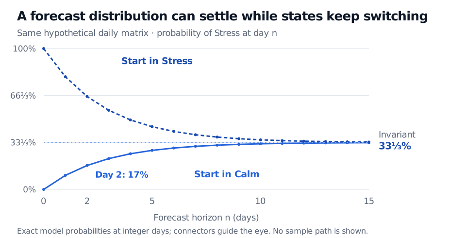
Exact Stress forecast probabilities under the hypothetical daily chain approach one third. Starting in Calm the probability rises from zero to 17% at day 2; starting in Stress it falls from 100%. Both approach the invariant 33 and one third percent.

Exact forecast distributions at integer days, with connectors to guide the eye. These curves show probabilities across possible outcomes, not a realised regime path.

The conditions matter. A chain that switches states with certainty every day has stationary weights $(1/2,1/2)$ , but starting in one state makes its distribution alternate forever. An identity transition matrix leaves every initial distribution unchanged, so stationarity is not unique. For countably infinite chains, irreducibility alone does not guarantee a stationary probability distribution; positive recurrence is needed.

In the finite irreducible example, long-run time fractions also approach the stationary weights almost surely. That does not fix the fraction on a short realised path or make each future day “one-third stressed.” If transition probabilities change or the chosen state omits predictive information, the fixed-matrix forecast and its limiting weights need reassessment.

For a fuller development, Markov Chains — Transition Matrices and the Markov Property covers transition diagrams, credit-rating states and expanding the state to retain history. The full lesson requires membership; its public page provides a preview.

Sources

Richard Durrett, Essentials of Stochastic Processes, third edition (2016), §§1.1–1.4 and §1.6, especially Theorems 1.19–1.22: transition laws, stationary distributions, convergence and long-run frequencies.
Dimitri P. Bertsekas and John N. Tsitsiklis, Introduction to Probability, second edition (2008), §§7.1–7.3: finite discrete-time chains, state classification and steady-state behaviour.
Stephen Boyd and Lieven Vandenberghe, Introduction to Applied Linear Algebra — Vectors, Matrices, and Least Squares, §9.1: state evolution as a linear dynamical system and retaining finite history through an enlarged state.
Stanford University, Stats 366 / Stats 166: Markov Chains: conditional-state dependence and powers of a transition matrix.

What the current state tells you

A risk forecast with two possible regimes

An invariant distribution is a different question

Sources

Related terms

Conditional probability

Independence

Stochastic process