Transition kernel: Definition & Examples

A transition kernel assigns a probability distribution for the next state to each possible current state, with a measurability condition that makes those assignments usable in probability calculations. It is the object behind a credit-migration table, a regime-switching model or a continuous-state forecast.

The input is a state; the output is a whole probability law. Asking for tomorrow's expected risk score uses only one feature of that law. Asking for the chance of crossing a limit requires the probabilities the kernel assigns to sets of outcomes.

Read the two arguments separately

On a measurable state space $(E,\mathcal{E})$ , a transition kernel is a map

P:E\times\mathcal{E}\longrightarrow[0,1]

with two requirements:

For each fixed state $x$ , the assignment $A\mapsto P(x,A)$ is a probability measure: it is countably additive, gives the empty set probability zero and satisfies $P(x,E)=1$ .
For each fixed measurable set $A$ , the function $x\mapsto P(x,A)$ is measurable. In particular, evaluating it at a random current state produces a measurable random quantity.

Thus

x

is where the system starts, while

A

is a collection of destinations. The second requirement allows the forecast to be averaged over an uncertain starting state. Drapeau's definition treats this probability kernel as a special case of a measure-valued kernel.

For a homogeneous discrete-time Markov chain, the forecasting interpretation is

\mathbb{P}(X_{n+1}\in A\mid\mathcal{F}_n) =P(X_n,A)\quad\text{almost surely},

where

\mathcal{F}_n

is the specified information through time

n

. The Markov property justifies using the current state to summarize that information. A kernel is a mathematical assignment; choosing one for a model does not establish that observed market data satisfy this property.

A transition matrix is the finite version

Suppose a hypothetical daily risk regime has two states, Calm and Stress. With rows and columns ordered Calm, Stress, let its transition matrix be

M=\begin{pmatrix}0.8&0.2\\0.3&0.7\end{pmatrix}.

Starting in Calm, tomorrow is Stress with probability $P(\text{Calm},\{\text{Stress}\})=0.2$ . Tomorrow is somewhere in the state space with probability

P(\text{Calm},\{\text{Calm},\text{Stress}\})=0.8+0.2=1.

More generally, $P(i,A)=\sum_{j\in A}M_{ij}$ . A matrix stores the probabilities of singleton destination sets; summing the relevant entries recovers every event probability. All subsets are measurable here, so the measurability condition adds no difficulty.

These numbers are model assumptions, not estimated migration frequencies. The SelfMadeQuant lesson Multistep Transition Probabilities and the Chapman–Kolmogorov Equations develops the finite-state calculations behind longer-horizon forecasts (membership for the full lesson; public preview).

A continuous state needs probabilities of regions

Now replace the regime label with a dimensionless risk score. Consider the illustrative autoregressive model

X_{n+1}=0.5X_n+\varepsilon_{n+1}, \qquad \varepsilon_{n+1}\sim\mathcal{N}(0,1),

with independent innovations, each independent of the history available at the current step. Conditional on

X_n=x

, the next score has normal distribution

\mathcal{N}(0.5x,1)

. Writing

\phi

for the standard normal density, its kernel is

P(x,A)=\int_A\phi(y-0.5x)\,dy, \qquad A\in\mathcal{B}(\mathbb{R}).

Here $\mathcal{B}(\mathbb{R})$ denotes the Borel sets, which include intervals and their countable combinations. Joint measurability of the normal density makes this a measurable assignment in $x$ .

Fix the event

A=(1,\infty)

: tomorrow's score exceeds 1. With

\Phi

the standard normal cumulative distribution function,

P(x,(1,\infty))=1-\Phi(1-0.5x).

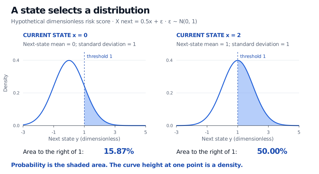
At current score

x=0

, the exceedance probability is

1-\Phi(1)\approx0.1586553

, or 15.87%. At

x=2

, the next-state mean is exactly the threshold 1, so the probability is 50% by symmetry.

Two conditional normal densities for the dimensionless model X next equals 0.5x plus standard normal noise. At current state 0, the next-state mean is 0 and the probability above 1 is 15.87%. At current state 2, the mean is 1 and the probability above 1 is 50%. Both conditional standard deviations are 1.

An exact hypothetical Gaussian model. Changing the current state shifts the conditional distribution; the shaded area gives the probability of the same destination set, $(1,\infty)$ .

The probability density

p(x,y)=\phi(y-0.5x)

is not the probability of landing exactly at

y

. This model has

P(x,\{y\})=0

for every single

y

, even where its density is positive. A transition kernel need not have a density with respect to length on the real line. The kernel concept also covers discrete laws and deterministic moves. For a deterministic measurable update

T

, for example,

P(x,A)=\mathbf{1}_A(T(x))

concentrates all probability at

T(x)

Carry the whole law through the next step

The Chapman–Kolmogorov equations compose transition kernels by averaging over the intermediate state. For the same one-step kernel at every step,

P^2(x,A)=\int_E P(y,A)\,P(x,dy).

The notation $P(x,dy)$ means integrate against the probability measure selected by $x$ . It does not assume a density. The integral becomes a sum in the finite model: the two-day probability of Stress starting from Calm is

0.8(0.2)+0.2(0.7)=0.30.

In the Gaussian model, substituting the first update into the second gives

X_{n+2}=0.25x+0.5\varepsilon_{n+1}+\varepsilon_{n+2} \quad\text{given }X_n=x.

Independent normal innovations therefore give the two-step law $\mathcal{N}(0.25x,1.25)$ . This is the same law obtained by integrating over the intermediate score; the second shock has not replaced the uncertainty from the first one.

Time homogeneity is an additional assumption. A general Markov model uses

P_{s,t}(x,A)

for the transition from time

s

to time

t

. For

s<u<t

, its composition rule is

P_{s,t}(x,A)=\int_E P_{u,t}(y,A)\,P_{s,u}(x,dy).

Only in a time-homogeneous model does this depend on elapsed time

t-s

rather than the calendar starting time. A fixed daily matrix and the fixed-coefficient Gaussian example both impose homogeneity. Calendar-dependent transition laws require their own kernels. Shalizi's lecture develops this composition and the distinction between general and homogeneous transition families.

For risk forecasting, this is the practical benefit of the kernel viewpoint: the same operation propagates uncertainty through discrete regimes, continuous scores or mixtures of both. The modeller must still choose a sufficient state, an appropriate time horizon and a defensible transition law.

Sources

Samuel Drapeau, Stochastics: Markov Processes, “From Markov Process to Transition probability.” Measurable kernels, probability measures and regular conditional distributions on Borel spaces.
Richard Durrett, Essentials of Stochastic Processes, third edition, Springer, 2016, Sections 1.1–1.2. Homogeneous finite-state chains, row-stochastic matrices and multistep transition probabilities.
Cosma Rohilla Shalizi, Markov Processes, Chapter 9, 36-754 lecture notes, Carnegie Mellon University, 2006, Section 9.2. Products of probability kernels and homogeneous transition families.

Read the two arguments separately

A transition matrix is the finite version

A continuous state needs probabilities of regions

Carry the whole law through the next step

Sources

Related terms

Cumulative distribution function

Markov chain

Markov property

Normal distribution

Probability density function

Transition matrix