Read a row-stochastic transition matrix, propagate a regime forecast and see why two steps require matrix multiplication rather than squaring entries.
Transition matrix
A transition matrix is a table of probabilities for moving between states in one specified time step. In a Markov chain, it supplies the state-dependent rule used to forecast future regimes, credit ratings or queue lengths.
Here we use the row convention: row i is the current state, column j is the next state, and
Pij=P(Xt+1=j∣Xt=i).
Each entry is a conditional probability. Every entry must be nonnegative and every row must sum to one. Such a matrix is called row-stochastic. A matrix alone does not specify today's state distribution; that is a separate input to the forecast.
Read a row, then move the distribution
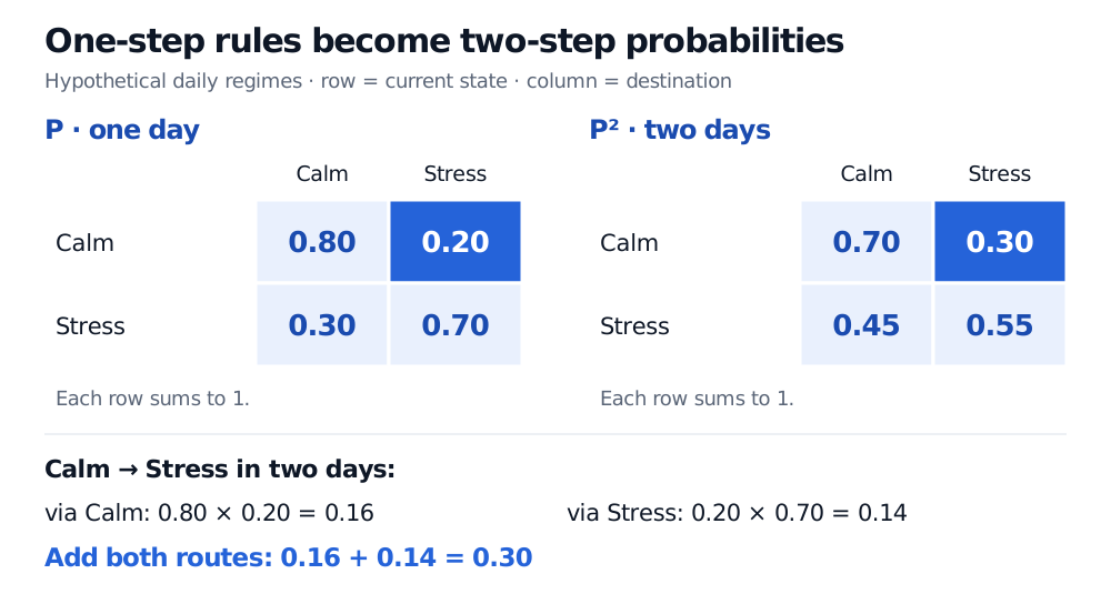
Suppose a hypothetical market model has two regimes, Calm and Stress, ordered this way in both rows and columns. Its stipulated daily matrix is
P=(0.800.300.200.70).
These are illustrative model probabilities, not estimates from market data. From Calm, tomorrow is Stress with probability 0.20. From Stress, tomorrow is Stress with probability 0.70. The diagonal entries are one-day stay probabilities; neither state is an absorbing state, which would require its diagonal entry to be one.
Write today's probabilities as a row vector qt. The next day's distribution is
qt+1=qtP,qt+1,j=i∑qt,iPij.
If today is definitely Calm, q0=(1,0), so q1=(0.80,0.20). If today's state is uncertain with q0=(0.60,0.40) instead, tomorrow's Stress probability is 0.60(0.20)+0.40(0.70)=0.40. That marginal probability averages over today's possible states; it is neither of the matrix's conditional Stress entries.
Some texts store distributions as columns. With the same row-stochastic P, their update is qt+1T=PTqtT. Alternatively, they may define a column-stochastic transition matrix from the outset. Check the convention before multiplying.
Two days means matrix multiplication
Assume the model is time-homogeneous: the same one-day rule applies at each date. Then
P2=PP=(0.700.450.300.55).
The Calm-to-Stress entry includes both possible intermediate regimes:
Multiplication follows each route; addition combines mutually exclusive routes with the same endpoint. This is the Chapman–Kolmogorov equation in matrix form. Squaring the single entry 0.20 gives 0.04, which is not the two-day Calm-to-Stress probability: the second transition depends on the intermediate state.
One-day matrix rows are Calm: 0.80, 0.20; Stress: 0.30, 0.70. Two-day rows are Calm: 0.70, 0.30; Stress: 0.45, 0.55. Two routes from Calm to Stress contribute 0.16 and 0.14, summing to 0.30.
Hypothetical daily regime model. Both matrices retain unit row sums; the highlighted endpoint combines paths through either intermediate regime.
Starting definitely Calm gives q2=q0P2=(0.70,0.30). More generally, qn=q0Pn, including P0=I for the zero-step forecast. Nonnegative matrix products preserve total probability because each destination sum uses rows whose mass is one.
A time step is part of the model
A daily matrix and an annual rating transition matrix answer different questions. Label the interval, state order and probability interpretation alongside the numbers. For credit-risk forecasting, historically estimated migration probabilities are not automatically the risk-neutral probabilities required for pricing.
Time-homogeneity also matters separately from the Markov property. If Pt governs the move from date t to t+1, a time-varying Markov model uses
qn=q0P0P1⋯Pn−1.
Keep those factors in chronological order under the row convention; matrices generally do not commute. A single power of a fixed matrix is justified only when that repeated transition rule is the intended model. Valid row sums alone do not establish that a chosen market state captures all predictive history or that estimated probabilities will remain stable.
Richard Durrett, Essentials of Stochastic Processes, third edition (2016), §§1.1–1.2: row-stochastic matrices, time-homogeneity and multistep transition probabilities.
Susan Holmes, Stanford University, Stats 366 / Stats 166: Markov Chains: conditional transition entries, matrix powers and row-vector propagation.