Summarise observed returns with explicit units, weights and variance divisors, and see why descriptive summaries do not establish future performance or preserve time order.
Descriptive statistics
Descriptive statistics summarises the data actually observed, using numbers, tables and charts. In a trading report, it answers questions such as “What was the average daily return in this window?” and “How widely did those returns vary?” It does not, by itself, establish the strategy's expected future return.
The observations may be a sample from a larger population, or the entire finite collection of interest. Description is possible in either case. Statistical inference goes further: it uses observations and assumptions to draw conclusions about an unobserved population or generating process, with uncertainty attached.
Six days on a performance report
Suppose a synthetic strategy has these six daily simple total returns, after the costs included in its stipulated return series:
−2%,−1%,0%,1%,2%,10%.
Each day receives equal weight. These are consecutive daily observations, not six equally likely future scenarios. For calculation, write their percentage-number values as x=(−2,−1,0,1,2,10): one unit on this scale is one percentage point (pp).
Summary
Value
What it describes
Observation count
6 days
Size of the recorded window
Arithmetic mean
1.666667% per day
Equal-weight average daily return
Median
0.5%
Midpoint of the ordered central returns, 0% and 1%
Minimum / maximum
−2% / 10%
Observed extremes
Range
12 pp
Distance between the extremes
Sample variance, divisor 5
18.666667 pp²
Squared dispersion around the mean
Sample standard deviation
4.320494 pp
Dispersion in the original return units
The sample mean is 10/6=5/3 on the percentage-number scale. The 10% day pulls it above the median. Removing that day would make the mean of the remaining five days zero. That is a sensitivity check, not permission to discard a valid large gain. Check the record before deciding whether an extreme is an error or real performance.
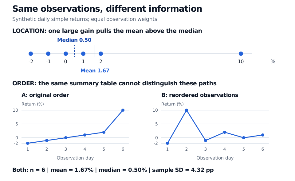
Six synthetic daily returns range from −2% to 10%; mean 1.67%, median 0.50% and sample standard deviation 4.32 percentage points. Two different daily orderings have identical summaries.
The upper plot shows why location summaries differ. The lower plots preserve the same six values but change their order; neither the mean nor standard deviation records that change.
State the divisor and the units
For n observations, the arithmetic mean and sample variance are
xˉ=n1i=1∑nxi,s2=n−11i=1∑n(xi−xˉ)2,n≥2.
Here the squared deviations sum to 280/3 pp². Dividing by five gives s2=56/3 pp². The standard deviation is its square root, about 4.320494 pp. This measures the spread of daily observations; it is not the standard error of their mean.
A second legitimate descriptive convention divides the same sum by n. It gives 140/9≈15.555556 pp², the variance of the empirical distribution that puts equal mass on each recorded observation. If these six days are the whole finite population being described, this is its population variance. Neither divisor discovers the variance of future returns. The familiar unbiased-estimation justification for n−1 requires, for example, independent, identically distributed observations with finite variance; computing the summary itself does not require independence.
Software units matter too. If returns are stored as decimals, use (−0.02,−0.01,0,0.01,0.02,0.10). Standard deviation is then about 0.04320494; variance is about 0.001866667 in squared decimal-return units. Scaling returns by 100 scales standard deviation by 100 and variance by 10,000. Label a 12 pp range as a difference in returns, rather than a 12% relative increase.
What a compact summary leaves behind
Averages and dispersion compress information. These particular summaries are unchanged by reordering the observations, so they cannot reveal trends or volatility clustering in a time series. Retain a dated return plot; for a larger sample, add a histogram to inspect shape. Six observations provide little basis for judging tail behaviour.
The arithmetic daily mean also differs from compounded growth. Over consecutive periods, simple returns compound through ∏i(1+ri), with ri in decimal units. A positive average is not a substitute for computing the realised investment outcome with the correct cash-flow and cost treatment.
Before comparing two reports, match the asset universe, currency, date window, daily versus monthly horizon, simple versus log returns, and equal versus capital weights. Record missing observations and adjustments for dividends, splits and stale prices. A precise average of a selected or corrupted dataset precisely describes that dataset, not necessarily the investment opportunity you meant to study. Annualising volatility or attaching confidence intervals adds assumptions beyond this descriptive table.
For a first extension, Basic Statistics and Regression connects these summaries to sampling uncertainty and paired observations (free with a signed-in account; public preview available). Financial Return Characteristics develops return conventions, tails and dependence (membership; public preview available).
Sources
John A. Rice, Mathematical Statistics and Data Analysis, 3rd ed., §§10.4–10.6: location, dispersion and graphical summaries.