Distinguish approaching a solution from merely stopping, read quadratic convergence in exact Newton iterates, and separate iteration error from grid and rounding error.
Convergence of a numerical method
Convergence of a numerical method means that its approximations approach the intended mathematical solution as the relevant computational limit is taken. For an iterative solver, that limit is usually an increasing number of iterations. For a discretisation, it is usually a shrinking grid spacing or time step.
A bond-yield solver can stop changing its answer without having found the yield. A pricing grid can be solved very accurately while still being too coarse. Convergence is therefore a claim about a specified target and a specified limiting process, rather than a synonym for “the program finished.”
What is approaching what?
In root-finding, let x∗ be the desired root and xk the approximation after k iterations. Convergence means
k→∞limEk=0,Ek=∣xk−x∗∣.
For vectors, replace the absolute value by a stated norm. A maximum-component error and an average squared error answer different questions; the norm and units belong in a convergence report.
For a finite-difference method, write the approximation as uh, where h measures grid spacing. After defining how the numerical and exact solutions are compared, convergence means ∥uh−u∥→0 as h→0. Other error sources must also be controlled: refining the spatial grid alone need not remove time-stepping or boundary-truncation error. A converged inner solver delivers the solution of the discretised equations; grid convergence asks whether those equations approximate the continuous problem. Driscoll and Braun’s finite-difference discussion develops the grid-spacing interpretation.
Watching an error square itself
Consider the dimensionless equation f(x)=x2−2=0, with target x∗=2. Newton–Raphson gives
xk+1=21(xk+xk2).
Starting at x0=3/2, the first iterates can be kept as exact fractions:
Iteration k
Exact iterate xk
Absolute error Ek, rounded
0
3/2
8.579×10⁻²
1
17/12
2.453×10⁻³
2
577/408
2.124×10⁻⁶
3
665857/470832
1.595×10⁻¹²
The falling errors suggest a rate; algebra identifies it. With the signed error ek=xk−2,
ek+1=2xkxk2+2−22xk=2xkek2.
Here every iterate stays above 2 and below its predecessor. Its positive limit must satisfy x=(x+2/x)/2, so it is 2. Consequently,
Ek2Ek+1⟶221≈0.353553.
This is quadratic convergence: once the error is small, the next error is roughly a constant times its square. It explains the rough doubling of correct digits near the solution.
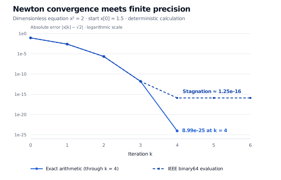
Exact Newton errors reach 8.99e-25 at step 4, while binary64 stagnates near 1.25e-16.
Original deterministic calculation: exact rational Newton iterates compared with the update (x+2/x)/2 evaluated in IEEE binary64. Errors use a separately checked high-precision square-root reference; the exact-arithmetic curve is shown only through step 4.
Rate, domain and arithmetic are separate claims
Linear convergence typically has Ek+1/Ek→q with 0<q<1: each iteration removes a roughly fixed fraction of the remaining error. Quadratic convergence has Ek+1/Ek2→C with 0<C<∞. For bisection with a continuous function and reliable endpoint signs, the retained bracket width halves per step; its midpoint error is bounded by half that width. This is linear contraction. These rates describe eventual behaviour; early iterations of other methods need not follow their asymptotic rate. An error that decreases at every step is not required for convergence either.
For a sufficiently smooth function with a simple root, Newton’s quadratic convergence is a local result: the starting guess must be sufficiently close. It is not a promise from every initial value. A zero derivative can make a step undefined, and an iteration may leave the admissible domain or approach a different root. NIST §3.8 states the local result and distinguishes simple from multiple roots.
The same word “order” is also used for grid error. If E(h)≈Ch2 in the asymptotic regime, halving h cuts that error by about four. This is second-order grid accuracy; it does not mean the iterative relation Ek+1≈CEk2. Specify which variable is changing before interpreting a convergence rate.
Finally, the ideal limit usually assumes exact arithmetic. In the figure, the binary64 calculation eventually repeats the same stored value. The step is zero although the forward error remains about 1.25×10⁻¹⁶. Extra iterations cannot recover the exact-arithmetic error of about 8.99×10⁻²⁵ at step 4. Floating-point arithmetic places a practical floor on this example; other problems may stagnate much earlier through rounding, poor conditioning or inaccurate function evaluations. The Python floating-point guide explains why stored values and displayed decimals differ.
Deciding when an answer is adequate
In a real calculation, x∗ is usually unknown. Three observable checks help, but have different meanings:
A small step ∣xk+1−xk∣ measures movement. It can signal convergence or stagnation.
A small residual∣f(xk)∣ measures how well the equation is satisfied. It is not automatically a bound on error in xk.
An error certificate, when available, translates those observations into a guarantee. For a scalar differentiable f, if ∣f′(x)∣≥m>0 throughout the interval joining xk to the root, the mean value theorem gives ∣xk−x∗∣≤∣f(xk)∣/m.
For an implied-volatility equation, the residual is a price difference while the unknown is volatility. Dividing by the local price sensitivity gives a first-order volatility-error estimate near a simple root; a rigorous bound needs control of that sensitivity over an interval. Low vega can make a small pricing residual compatible with a much larger volatility error. This is where numerical conditioning enters the stopping decision.
Choose numerical tolerances in the units of the quantity that matters, monitor failure as well as success, and retain an iteration cap. A finite table of improving values supports a convergence diagnosis; it does not prove the limiting claim for every allowed input.
For the finance applications behind both limits, SelfMadeQuant’s Root-Finding and Numerical Integration applies iteration to bond yield and discretisation to expectations. The full lesson requires membership; the linked outline and introduction are public.